Okhsv and Okhsl
Two new color spaces for color picking
This post has an accompanying interactive comparison of color pickers.
I would recommend checking out the interactive demo first, then return if you are interested in the background and technical details.
Picking colors is a common operation in many applications and over the years color pickers have become fairly standardized. Ubiquitous today are color pickers based on HSL and HSV. They are simple transformations of RGB values to alternative coordinates chosen to better correlate with perceptual qualities.
Here are two common variants of color pickers built on HSL and HSV:
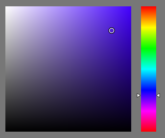
A HSV color picker.
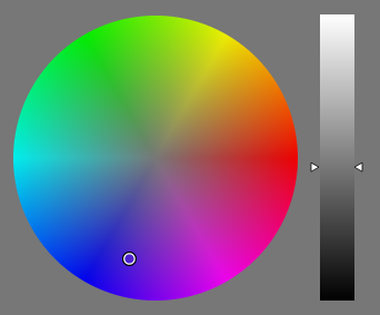
A HSL color picker.
Despite color picking playing a big role in a lot of applications, the design of color pickers isn’t a particularly well researched topic. While some variation exist in the widgets themselves, the choice of HSL or HSV is mostly taken for granted, with only a few exceptions.
Is their dominance well deserved or would it be possible to create better alternatives? I at least think that this question deserves to be explored and that color picker design should be an active research topic. With this post I hope to contribute to the exploration of what a better color picker could and should be, and hopefully inspire others to do the same!
The main focus here will be on the choice of color space, rather than the design of the UI widget used for navigating the color space.
This rest of this post is organized as follow:
- A brief history of color picking
- What are meaningful properties of color spaces for color picking?
- What options exist already and how do they perform?
- Introducing two new color spaces: Okhsl and Okhsv
- Ideas for future work
Color picking before computers
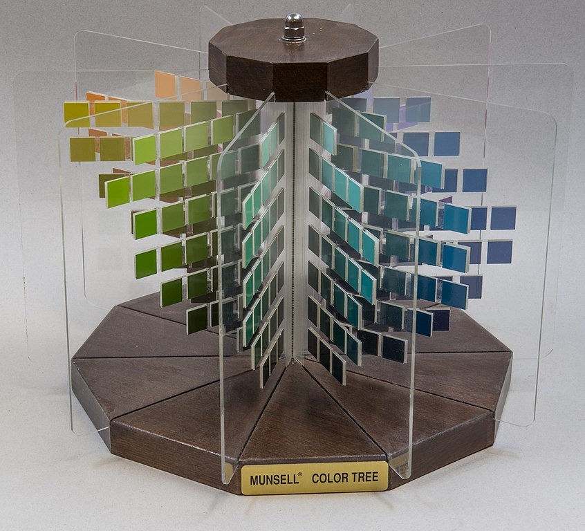
Munsell Color System. Photo by Hannes Grobe, license CC BY-SA 4.0
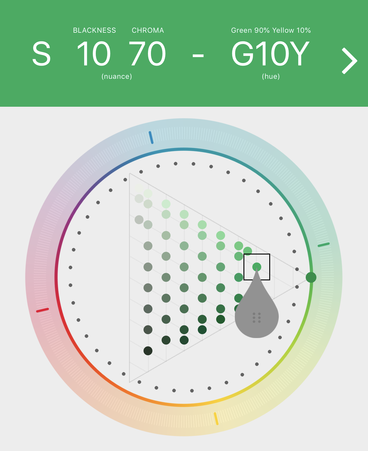
Example of NCS color picker. Screenshot from NCS Navigator in the Colourpin app.
Categorizing, describing and picking colors is an old problem and predates computers by many centuries. Over the years countless artists and scientists have worked to understand how humans perceive colors and used that knowledge to try and create practical systems for describing colors. Many different color ordering systems have been created over the years based on mixing properties of paints, light or on perceptual qualities.
During the 20th century two important color systems emerged. The Munsell Color System and the Natural Color System (NCS). Both of them are based on human perception and were derived using experiments, but with different approaches. The two systems are used in many practical applications today still.
In the Munsell color system, colors are described with three parameters, designed to match the perceived appearance of colors: Hue, Chroma and Value. The parameters are designed to be independent and each have a uniform scale. This results in a color solid with an irregular shape. Modern color spaces and models, such as CIELAB, Cam16 and my own Oklab, are very similar in their construction.
The Natural Color System takes a different approach, and is designed to make it easy to describe colors, rather than to match perceptual qualities. It does this by describing colors by their similarity to six primary colors: white, black, yellow, red, green and blue. The yellow, red, green and blue colors are used to determine the hue. The final color is described by a color triangle with the corners white, black and the most saturated color of the given hue. A position in the triangle is described with the parameters whiteness, blackness, chromaticness. Any two of those parameters are sufficient, since they sum to one.
For more information about historical color systems, this is a great resource: colorsystem.com.
What makes a good color picker?
Before diving into how color pickers have evolved in the digital era, let’s look a bit further at what considerations can be relevant when designing a color space for color picking. This part assumes familiarity with color appearance concepts such as lightness, chroma, saturation and hue.
In this post the focus will be on what is today the most common case, picking colors in the sRGB gamut. Wide gamut and HDR displays are becoming more common and will be increasingly important, so wide gamut and HDR color picking is definitely a topic for further research and development, but it will not be considered here.
Here’s an attempt at capturing useful properties for color spaces designed for picking colors:
- Orthogonal Lightness - Hue/Chroma/Saturation can be altered, while keeping perceived Lightness constant
- Orthogonal Chroma - Lightness/Hue can be altered, while keeping perceived Chroma constant
- Orthogonal Saturation - Lightness/Hue can be altered, while keeping perceived Saturation constant
- Orthogonal Hue - Lightness/Chroma/Saturation can be altered, while keeping perceived Hue constant
- Simple Geometrical Shape - Fit the target gamut into a cylinder or other simple shape, so that parameters can be altered independently without resulting in colors outside the target gamut. Could also be a swept triangle like NCS, since it is simple to map back and forth to a cylinder.
- Max Chroma at edge - Make it easy to find the strongest color of a given hue, by placing the strongest color on edge of the color volume.
- Varies Smoothly - Vary smoothly with each parameter. No discontinuous or abrupt changes.
- Varies Evenly - The perceived magnitude of the change in color caused by changing a parameter should be uniform for all values of the parameter.
Note: These properties are in conflict, so designing a color space for color picking is a about finding which tradeoffs to make. In particular, independent control of hue, lightness and chroma can not be achieved in a color space that also maps sRGB to a simple geometrical shape.
Color spaces for color picking
By far the most used color spaces today for color picking are HSL and HSV, two representations introduced in the classic 1978 paper “Color Spaces for Computer Graphics”. HSL and HSV designed to roughly correlate with perceptual color properties while being very simple and cheap to compute.
Worth noting is that HSL and HSV are not quite color spaces on their own, they are transformations from a source RGB color space. For each set of RGB primaries and transfer functions, the transformation to HSL and HSV produces unique color spaces. Today HSL and HSV are most commonly used together with the sRGB color space, so that is what we will look at here and we will here use HSL and HSV to refer to HSL and HSV for the sRGB color space.
Also useful to note is that HSL and HSV are not continuously differentiable, so that limits their use with numerical optimization and machine learning.
HSV
HSV describes colors with three parameters:
- "Hue" - Roughly corresponds to perceived hue, but it has quite severe distortions.
- "Saturation" - Roughly corresponds to saturation relative to maximum possible saturation in sRGB of the same hue.
- "Value" - A bit hard to define. Can be seen as how much to mix the color with black, with 100% being no black and 0% completely black. “Value” is sometimes also referred to as Brightness.
HSV is quite similar to the Natural Color System in its structure and it’s possible to transform it to have parameters more similar to NCS, then referred to as hue, whiteness and blackness (HWB). After that transformation the largest difference compared with NCS are:
- NCS is derived based on research into the appearance of colors and does a good job at matching human perception
- HWB/HSV has a simple construction, not taking research into color appearance into account and is not matching perception closely. Hue is the most problematic.
- NCS has a gamut designed to contain pigments realizable in paint/print
- HWB/HSV has a gamut based on the RGB color space it is constructed from (most commonly sRGB)
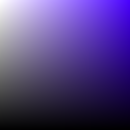
Example of hue distortion for deep blue colors. Notice the purple shift as saturation decreases.
HSL
HSV describes colors with three parameters:
- "Hue" - Identical to “hue” in HSV, with the same issues.
- "Saturation" - Roughly the chroma of the color relative to the most colorful color with the same “lightness” and “hue”. Confusingly referred to as saturation, which it is not comparable to. In the original paper it was referred to as “relative chroma”, which is more accurate. Not the same as “saturation” in HSV.
- "Lightness" - Some correlation with the perception of lightness, with 0% corresponding to black and 100% to white. Does not match the perception of lightness well at all for saturated colors. Referred to as “Intensity” in the original paper.
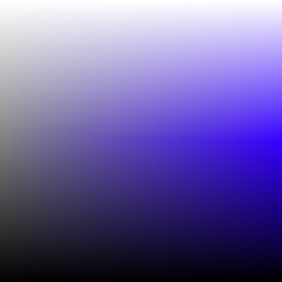
Example of hue distortion for deep blue colors.
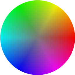
Example of colors HSL considers to have the same lightness.
HSLuv
HSLuv is a recent development to tackle some of the shortcomings of HSL. It is based on CIELChuv, a cylindrical form of 1976 CIE color space CIELUV. CIELChuv is constructed so that for a given hue, all colors of that hue can be constructed by additive blending of white and a saturated color of that hue (and in general, additive blending of light forms straight lines in CIELuv).
HSLuv describes colors with three parameters:
- "Hue" - Same as hue in CIELChuv. Does not match the perception of hue fully due to the Abney effect: the perception of hue does not correspond to additive blending.
- "Saturation" - Based on chroma as defined in CIELChuv, but rescaled to be relative to the most saturated sRGB color of the same “lightness” and “hue”.
- "Lightness" - Same as lightness in CIELChuv. Does a good job at matching perceived lightness.
Two drawback with HSLuv are:
- Does not match perception of hue. This is particularly obvious for deep blue and purple colors.
- The way “Saturation” is defined, it does not vary smoothly due to the uneven shape of the sRGB gamut. E.g. by keeping “Saturation” constant and changing hue, the perceived chroma can change drastically and abruptly.
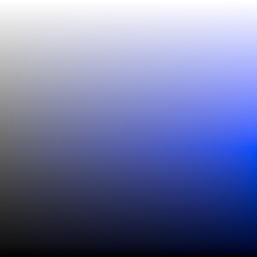
Example of hue distortion for blue colors. The distortion in HSLuv is different from that in sRGB and is caused by the Abney effect.
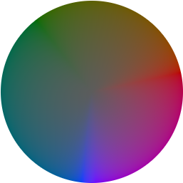
Example of constant lightness in HSLuv, with low “saturation” close to the center of the circle and maximum “saturation” at the edge. Notice how the blue and red hues are much more saturated than surrounding colors.
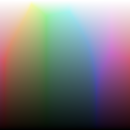
Slice of colors with constant “saturation” in HSLuv. The scaling to match the uneven shape of the sRGB gamut makes the perceived chroma vary unevenly.
Color spaces modelling color appearance
While there is a limited amount of research done regarding color picking, a lot of work has been done to create color models that are able to predict color appearance. These continue in the tradition of the Munsell color model discussed above, but use more modern color science and mathematical models to better model the appearance of color. One of the most famous of these is CIELab, but there are today several new models that perform better.
Comparing all the color models is beyond the scope of this post, the important conclusion here is that these models can model the perception of Lightness, Hue and Chroma much better than all the previously discussed options. For a brief overview of some of the more recent models, see my previous post “A perceptual color space for image processing”. Since then another color model has also appeared: ZCAM. For a much deeper overview of modern color science and different attempts at modeling color appearance, I recommend the book “Color Appearance Models” by Mark D. Fairchild.
The main drawback of using these models directly for color picking is that the sRGB gamut has a quite irregular shape in these color spaces. As a result, changing one parameter, such as hue, can easily create a color outside the target gamut, making them quite tedious to use. Several color pickers have been made using either CIELab or more modern lab-like color spaces. From what I can tell they have only seen limited use compared with the more common HSV and HSL color pickers however.
I would think that the reason that they haven’t caught on is that their drawbacks outweigh their benefits: using a space with parameters that don’t match the our perception of hue, lightness and chroma is easier than using one with an irregular shape. That is certainly my personal experience.
For the more advanced models an additional complication is that they have several parameters meant to be adjusted based on the viewing conditions. When used for color picking they seem to mostly be set to match some kind of average viewing conditions though.
Here are a couple of examples of the irregular shape of the sRGB gamut in a perceptual color space:
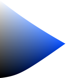
A slice of the gamut with a constant blue hue.
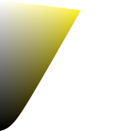
A slice of the gamut with a constant yellow hue.
It is unfortunately also common to see CIELab based color pickers showing colors outside the target gamut and often they are mapped back by simply clamping individual RGB components. This creates severe distortions in hue, lightness and chroma, in would would otherwise be a fairly uniform color space.
Summary
These are the color spaces I am aware of that are relevant, but please reach out if you are aware of any more color spaces useful for color picking.
To summarize, here is a table of the different color spaces discussed and how they match the different desirable properties. This is definitely a bit subjective, but will hopefully give a decent overview.
| HSV | HSL | HSLuv | Lab-like* | NCS | |
|---|---|---|---|---|---|
| Orthogonal Lightness | no | no | yes | yes | no |
| Orthogonal Chroma | no | no | no | yes | partial |
| Orthogonal Saturation | partial | no | no | no** | no |
| Orthogonal Hue | partial | partial | partial | yes | yes |
| Simple Geometrical Shape | yes | yes | yes | no | no*** |
| Max Chroma at Edge | yes | no | no | yes | no |
| Varies Smoothly | yes | yes | no | yes | yes |
| Varies Evenly | no | no | no | yes | partial |
*) This of course depends on which Lab-like color space. This is the best possible an appearance modelling color space could achieve.
**) If desirable, saturation can be used instead of Chroma, and then this would be a yes and “Orthogonal Chroma” a no.
***) NCS has a simple geometrical shape, but it does not match the sRGB gamut.
Finding a better tradeoff
One of the main advantages of HSL and HSV over the different Lab color spaces is that they map the sRGB gamut to a cylinder. This makes them easy to use since all parameters can be changed independently, without the risk of creating colors outside of the target gamut.
The main drawback on the other hand is that their properties don’t match human perception particularly well. Reconciling these conflicting goals perfectly isn’t possible, but given that HSV and HSL don’t use anything derived from experiments relating to human perception, creating something that makes a better tradeoff does not seem unreasonable.
We will attempt to do just that by creating new color spaces similar to HSL and HSV but that better match perception. This will be done by leveraging the Oklab color space. Using Oklab here over more advanced models such as CAM16 is useful because working out the math becomes a lot simpler. It also means that it won’t be a full color model able to adapt to different viewing conditions, but that is probably also desirable here since it is more practical.
For consistency with the naming of Oklab, these new color spaces will be called Okhsl and Okhsv. The parameters will also be referred to as , and and , and respectively. Those names are a bit confusing but I think making the new spaces easy to adopt for someone used to HSL and HSV is more important than trying to establish new names.
Intermission - a new lightness estimate for Oklab
One design decision with Oklab is to use a design that is scale independent. That is, Oklab has no concept of reference white, unlike CIELab for example. In many cases this is an advantage, since it makes dealing with larger dynamic ranges easier.
However, in the context of a color picker with well defined dynamic range and a clear reference white luminance it reduces Oklab’s ability to predict lightness. Therefore, an additional lightness estimate is needed to better handle these cases. With a reference white luminance of , the new lightness estimate is defined as:
With the inversion:
This new lightness estimate closely matches the lightness estimate of CIELab overall and is nearly equal at 50% lightness (Y for CIELab L is 0.18406, and 0.18419) which is useful for compatibility. Worth noting is that it is not possible to have a lightness scale that is perfectly uniform independent of viewing conditions and background color. This new lightness function is however a better tradeoff for cases with a well defined reference white.
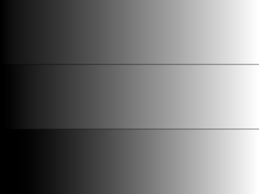
From top to bottom: CIELab , Oklab , Oklab .
Introducing two new color spaces: Okhsv and Okhsl
With this new lightness estimate, we are ready to look into the construction of Okhsv and Okhsl. Here is a rough overview of the general idea behind Okhsv and Okhsl and their construction. Some details are glossed over here, for all the details check out the source code below.
Okhsv
To derive Okhsv, we will start with OkLCh, use its estimate for hue, , as is and introduce and parameters that are calculated based on lightness, , and chroma, . To keep the triangular shape when using we also scale by .
Here is the sRGB gamut plotted for set of hues, with on the y-axis and on the x-axis:
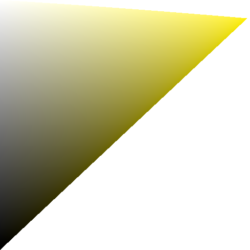
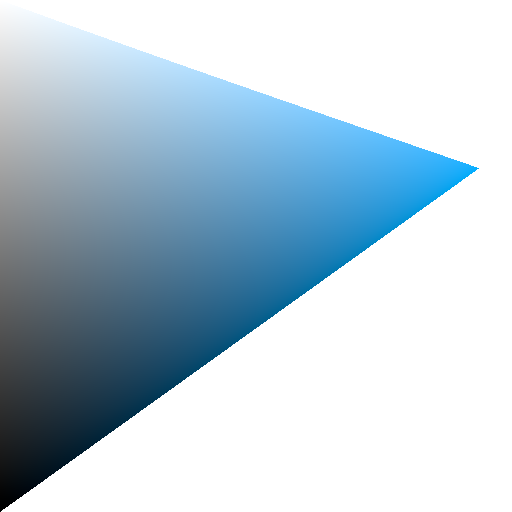
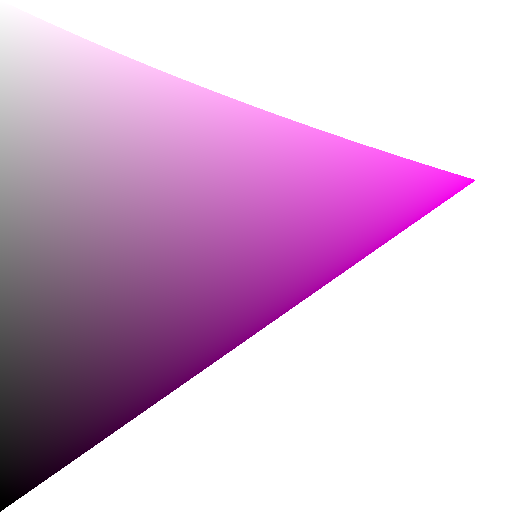
To create a HSV-like color space, we want to find a mapping so that the cusp of the triangle is in and . We also want to change the triangle shape into a square, by stretching the lower part of the triangle.
To find the cusp we can use the same method as in my previous post about sRGB gamut clipping.
If we perform this remapping we get the following result:
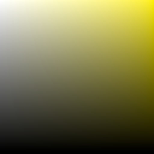
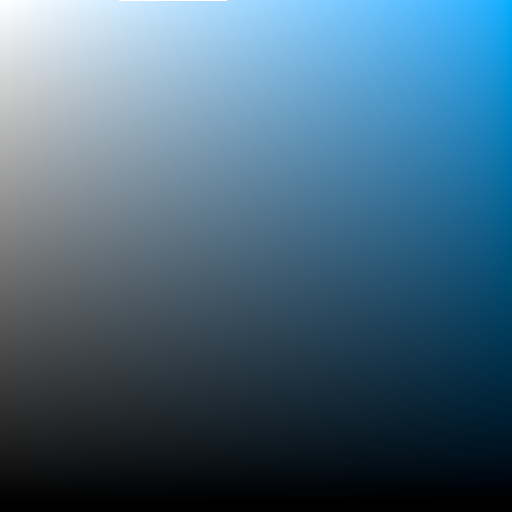
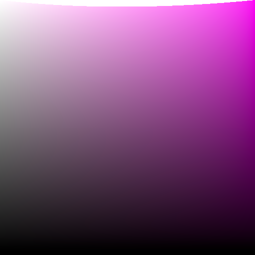
Remaining now is a small curve at the top, that we also have to remove. This is done by scaling to compensate. This step makes the space less uniform perceptually, but is needed to fit the sRGB gamut to a cylinder exactly. The change is quite small however. This gives the following result:
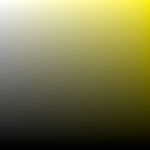
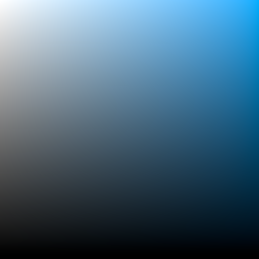
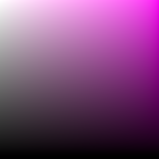
As an additional step we adjust saturation to be more uniform for low saturation colors. This makes it easier to compare saturation values for different colors, when saturation is low. The effect of this is subtle.
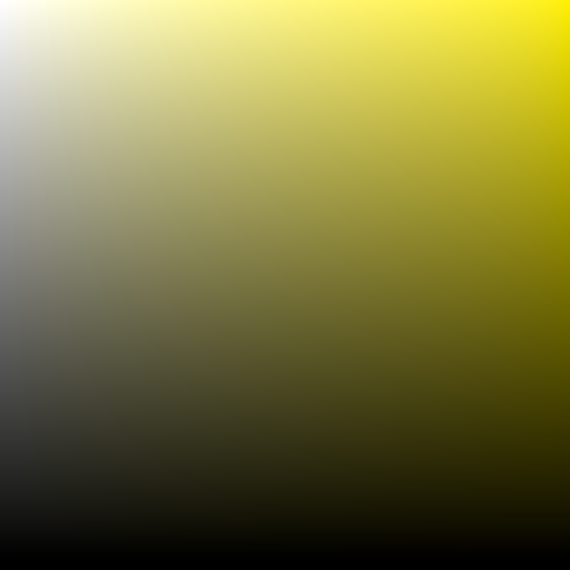

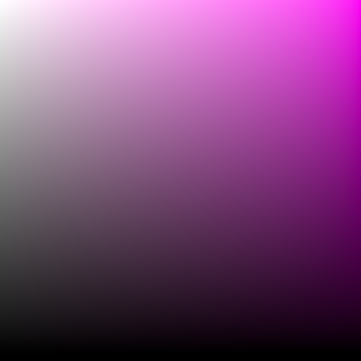
This gives us a new model with a simple geometrical shape and a hue parameter that closely matches perception. Overall the space will be very familiar to someone who is used to HSV, but with improved perceptual uniformity.
Okhwb
If desired, Okhsv can also be converted to a HWB (hue, whiteness and blackness) form.
With the inverse:
Okhsl
To derive Okhsl we also start with OkLCh. and are kept as is, with referred to as instead for consistency.
For we want to somehow remap so that the sRGB gamut nicely fits into a cylinder.
The simplest way to do this is to simply scale it by the maximum chroma inside the sRGB gamut for a given value of and , , which is what HSLuv does. As we have seen with HSLuv though, the unevenness of the shape of the gamut will affect the interior of the entire space resulting in an uneven scale for the component.
Instead it would be good if we could find a way to keep the unevenness local to colors close to the edge of the gamut, leaving the interior less affected. This is the key idea behind Okhsl.
One way to solve this would be to solve it as a boundary value problem, finding , with a boundary condition that and some set of differential equation that keeps the interior smooth. This approach could definitely give a good result and would be interesting to explore, but is likely to only have a numerical solution, which would make it hard to use practically to construct a color space.
Instead Okhsl uses a fairly ad-hoc approach to create a smoothly varying interior, since that makes it efficient to run and easy to invert.
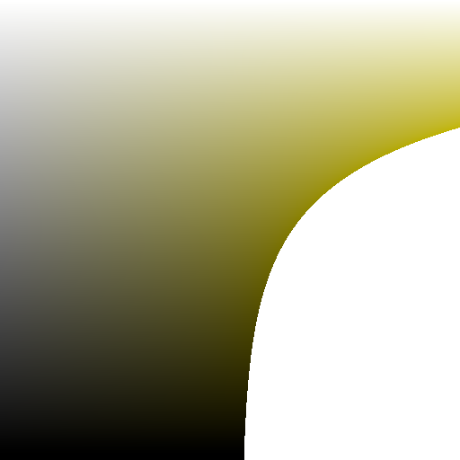
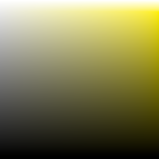
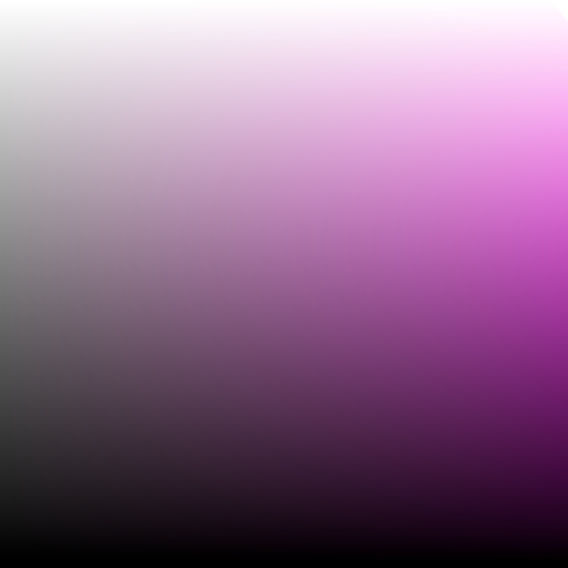
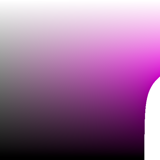
Instead of scaling by a single value for , the max possible value in the gamut, three different values are used, one for low values of , , one for midrange values of , and one for large values, . These are constructed the following way:
- is constructed to be independent of hue, this way creating continuity for colors close to the axis.
- is constructed to be closer in shape to , but still much smoother and has been constructed using an optimization process. See the source code for more details and the exact computation.
- is the maximum possible value for in the sRGB gamut for the given values of and
To get an understanding of , and , here are a few hue slices where is computed , and respectively.




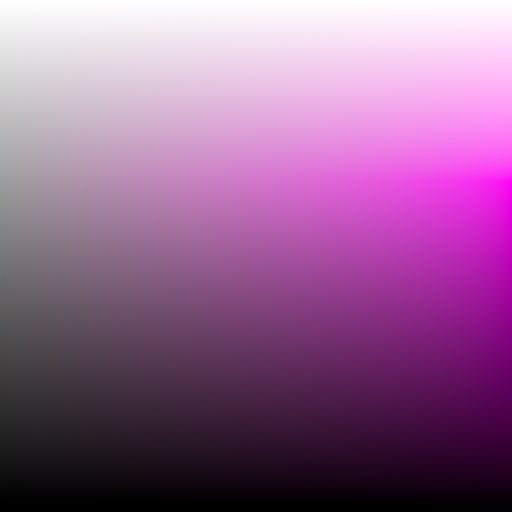
To create the full Okhsl model, the values are interpolated so that:
- At : ,
- At :
- At :
This gives the final Okhsl model:
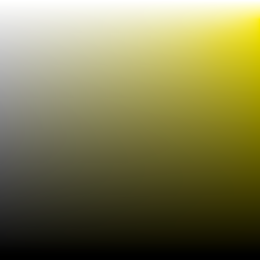

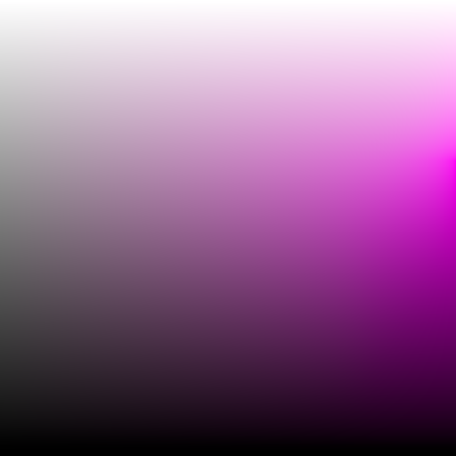
Altogether this gives a model with a simple geometrical shape that has parameters for lightness and hue that closely match perception. The model is quite different from regular HSL, in order to achieve a better lightness estimate. I believe Okhsl delivers a better overall compromise, and keeps many of the benefits of Lab-like color spaces, without the complexity of an irregular shape.
Here are a few examples of slices Okhsl, with constant lightness and saturation:
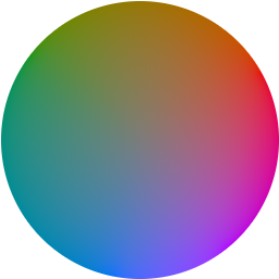
Example of constant “lightness” in Okhsl.
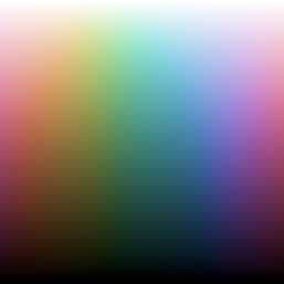
Slice of colors with constant “saturation” in Okhsl. While not matching perceived chroma fully it is smoothly varying.
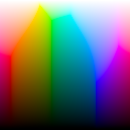
For 100% ‘saturation’ the variation in perceived chroma is larger, due to the shape of the sRGB gamut.
Summary
For completeness, here is a table of how Okhsv and Okhsl match the desired properties from earlier. Again, this is definitely a bit subjective. A better way to judge the performance is to just try the results yourself.
| Okhsv | Okhsl | |
|---|---|---|
| Orthogonal Lightness | no | yes |
| Orthogonal Chroma | no | no |
| Orthogonal Saturation | partial | no |
| Orthogonal Hue | yes | yes |
| Simple Geometrical Shape | yes | yes |
| Max Chroma at Edge | yes | no |
| Varies Smoothly | yes | yes |
| Varies Evenly | no | no |
Ideas for future work
Okhsv and Okhsl are my attempts at making better color pickers for the sRGB gamut. I would love to see more experimentation overall with color picker design and in the next few years, color pickers for wide gamut and HDR will be more and more important and need a lot of research. They both offer their own new challenges.
Wide gamut is challenging since we are seeing an increased variety of different gamuts. At least for a while, target color spaces will be much more varied and applications for authoring colors will have to either settle for common subset or have to deal with this complexity. This of course will have a big impact on what color pickers look like and how they behave.
One interesting avenue to pursue would be to more automatically create color spaces like Okhsv and Okhsl for a given color gamut. This would likely need to use a bit of a different approach, maybe using lookup tables and numerical solutions in order to not need as much handcrafted logic.
HDR also has the issue of not being quite standardized, but an added complexity is the increased dynamic range and variation is absolute brightness. In the past color pickers have been able to mostly ignore how the eye adapts to different luminance levels, but this does not work as well with HDR. So far the approaches I’ve seen are to use regular SDR color pickers, but with and added exposure/intensity control. Is this the best approach or are there new ways we should be working with HDR color pickers?
An additional thing to explore is what spacing of hues would be the best. Okhsl and Okhsv simply inherit their spacing from Oklab. A different option could be to do a remapping similar to NCS, which would make the parameter vary less evenly, but could make it easier to use by mapping the different axes to more familiar colors.
Source Code
Here is the Source Code for conversion between sRGB, HSL and HSV. This code depends on the code from my previous post sRGB gamut clipping, which is not included here. You can find the source for both posts combined here as a C++ header.
The interactive comparison of color pickers also has an implementation of this in JavaScript. The source is available here.
License
All the source code on this page is provided under the MIT license:
Copyright (c) 2021 Björn Ottosson

Permission is hereby granted, free of charge, to any person obtaining a copy of
this software and associated documentation files (the "Software"), to deal in
the Software without restriction, including without limitation the rights to
use, copy, modify, merge, publish, distribute, sublicense, and/or sell copies
of the Software, and to permit persons to whom the Software is furnished to do
so, subject to the following conditions:

The above copyright notice and this permission notice shall be included in all
copies or substantial portions of the Software.

THE SOFTWARE IS PROVIDED "AS IS", WITHOUT WARRANTY OF ANY KIND, EXPRESS OR
IMPLIED, INCLUDING BUT NOT LIMITED TO THE WARRANTIES OF MERCHANTABILITY,
FITNESS FOR A PARTICULAR PURPOSE AND NONINFRINGEMENT. IN NO EVENT SHALL THE
AUTHORS OR COPYRIGHT HOLDERS BE LIABLE FOR ANY CLAIM, DAMAGES OR OTHER
LIABILITY, WHETHER IN AN ACTION OF CONTRACT, TORT OR OTHERWISE, ARISING FROM,
OUT OF OR IN CONNECTION WITH THE SOFTWARE OR THE USE OR OTHER DEALINGS IN THE
SOFTWARE.
Common code
struct HSV { float h; float s; float v; };
struct HSL { float h; float s; float l; };
struct LC { float L; float C; };

// Alternative representation of (L_cusp, C_cusp)
// Encoded so S = C_cusp/L_cusp and T = C_cusp/(1-L_cusp)
// The maximum value for C in the triangle is then found as fmin(S*L, T*(1-L)), for a given L
struct ST { float S; float T; };

// toe function for L_r
float toe(float x)
{
	constexpr float k_1 = 0.206f;
	constexpr float k_2 = 0.03f;
	constexpr float k_3 = (1.f + k_1) / (1.f + k_2);
	return 0.5f * (k_3 * x - k_1 + sqrtf((k_3 * x - k_1) * (k_3 * x - k_1) + 4 * k_2 * k_3 * x));
}

// inverse toe function for L_r
float toe_inv(float x)
{
	constexpr float k_1 = 0.206f;
	constexpr float k_2 = 0.03f;
	constexpr float k_3 = (1.f + k_1) / (1.f + k_2);
	return (x * x + k_1 * x) / (k_3 * (x + k_2));
}

ST to_ST(LC cusp)
{
	float L = cusp.L;
	float C = cusp.C;
	return { C / L, C / (1 - L) };
}
HSV
This code converts between sRGB (not linear) and Okhsv.
struct HSV { float h; float s; float v; };
RGB okhsv_to_srgb(HSV hsv)
{
	float h = hsv.h;
	float s = hsv.s;
	float v = hsv.v;

	float a_ = cosf(2.f * pi * h);
	float b_ = sinf(2.f * pi * h);

	LC cusp = find_cusp(a_, b_);
	ST ST_max = to_ST(cusp);
	float S_max = ST_max.S;
	float T_max = ST_max.T;
	float S_0 = 0.5f;
	float k = 1 - S_0 / S_max;

	// first we compute L and V as if the gamut is a perfect triangle:

	// L, C when v==1:
	float L_v = 1     - s * S_0 / (S_0 + T_max - T_max * k * s);
	float C_v = s * T_max * S_0 / (S_0 + T_max - T_max * k * s);

	float L = v * L_v;
	float C = v * C_v;

	// then we compensate for both toe and the curved top part of the triangle:
	float L_vt = toe_inv(L_v);
	float C_vt = C_v * L_vt / L_v;

	float L_new = toe_inv(L);
	C = C * L_new / L;
	L = L_new;

	RGB rgb_scale = oklab_to_linear_srgb({ L_vt, a_ * C_vt, b_ * C_vt });
	float scale_L = cbrtf(1.f / fmax(fmax(rgb_scale.r, rgb_scale.g), fmax(rgb_scale.b, 0.f)));

	L = L * scale_L;
	C = C * scale_L;

	RGB rgb = oklab_to_linear_srgb({ L, C * a_, C * b_ });
	return {
		srgb_transfer_function(rgb.r),
		srgb_transfer_function(rgb.g),
		srgb_transfer_function(rgb.b),
	};
}

HSV srgb_to_okhsv(RGB rgb)
{
	Lab lab = linear_srgb_to_oklab({
		srgb_transfer_function_inv(rgb.r),
		srgb_transfer_function_inv(rgb.g),
		srgb_transfer_function_inv(rgb.b)
		});

	float C = sqrtf(lab.a * lab.a + lab.b * lab.b);
	float a_ = lab.a / C;
	float b_ = lab.b / C;

	float L = lab.L;
	float h = 0.5f + 0.5f * atan2f(-lab.b, -lab.a) / pi;

	LC cusp = find_cusp(a_, b_);
	ST ST_max = to_ST(cusp);
	float S_max = ST_max.S;
	float T_max = ST_max.T;
	float S_0 = 0.5f;
	float k = 1 - S_0 / S_max;

	// first we find L_v, C_v, L_vt and C_vt

	float t = T_max / (C + L * T_max);
	float L_v = t * L;
	float C_v = t * C;

	float L_vt = toe_inv(L_v);
	float C_vt = C_v * L_vt / L_v;

	// we can then use these to invert the step that compensates for the toe and the curved top part of the triangle:
	RGB rgb_scale = oklab_to_linear_srgb({ L_vt, a_ * C_vt, b_ * C_vt });
	float scale_L = cbrtf(1.f / fmax(fmax(rgb_scale.r, rgb_scale.g), fmax(rgb_scale.b, 0.f)));

	L = L / scale_L;
	C = C / scale_L;

	C = C * toe(L) / L;
	L = toe(L);

	// we can now compute v and s:

	float v = L / L_v;
	float s = (S_0 + T_max) * C_v / ((T_max * S_0) + T_max * k * C_v);

	return { h, s, v };
}
HSL
This code converts between sRGB (not linear) and Okhsl.
struct HSL { float h; float s; float l; };

// Returns a smooth approximation of the location of the cusp
// This polynomial was created by an optimization process
// It has been designed so that S_mid < S_max and T_mid < T_max
ST get_ST_mid(float a_, float b_)
{
	float S = 0.11516993f + 1.f / (
		+7.44778970f + 4.15901240f * b_
		+ a_ * (-2.19557347f + 1.75198401f * b_
			+ a_ * (-2.13704948f - 10.02301043f * b_
				+ a_ * (-4.24894561f + 5.38770819f * b_ + 4.69891013f * a_
					)))
		);

	float T = 0.11239642f + 1.f / (
		+1.61320320f - 0.68124379f * b_
		+ a_ * (+0.40370612f + 0.90148123f * b_
			+ a_ * (-0.27087943f + 0.61223990f * b_
				+ a_ * (+0.00299215f - 0.45399568f * b_ - 0.14661872f * a_
					)))
		);

	return { S, T };
}

struct Cs { float C_0; float C_mid; float C_max; };
Cs get_Cs(float L, float a_, float b_)
{
	LC cusp = find_cusp(a_, b_);

	float C_max = find_gamut_intersection(a_, b_, L, 1, L, cusp);
	ST ST_max = to_ST(cusp);

	// Scale factor to compensate for the curved part of gamut shape:
	float k = C_max / fmin((L * ST_max.S), (1 - L) * ST_max.T);

	float C_mid;
	{
		ST ST_mid = get_ST_mid(a_, b_);

		// Use a soft minimum function, instead of a sharp triangle shape to get a smooth value for chroma.
		float C_a = L * ST_mid.S;
		float C_b = (1.f - L) * ST_mid.T;
		C_mid = 0.9f * k * sqrtf(sqrtf(1.f / (1.f / (C_a * C_a * C_a * C_a) + 1.f / (C_b * C_b * C_b * C_b))));
	}

	float C_0;
	{
		// for C_0, the shape is independent of hue, so ST are constant. Values picked to roughly be the average values of ST.
		float C_a = L * 0.4f;
		float C_b = (1.f - L) * 0.8f;

		// Use a soft minimum function, instead of a sharp triangle shape to get a smooth value for chroma.
		C_0 = sqrtf(1.f / (1.f / (C_a * C_a) + 1.f / (C_b * C_b)));
	}

	return { C_0, C_mid, C_max };
}

RGB okhsl_to_srgb(HSL hsl)
{
	float h = hsl.h;
	float s = hsl.s;
	float l = hsl.l;

	if (l == 1.0f)
	{
		return { 1.f, 1.f, 1.f };
	}

	else if (l == 0.f)
	{
		return { 0.f, 0.f, 0.f };
	}

	float a_ = cosf(2.f * pi * h);
	float b_ = sinf(2.f * pi * h);
	float L = toe_inv(l);

	Cs cs = get_Cs(L, a_, b_);
	float C_0 = cs.C_0;
	float C_mid = cs.C_mid;
	float C_max = cs.C_max;

    // Interpolate the three values for C so that:
    // At s=0: dC/ds = C_0, C=0
    // At s=0.8: C=C_mid
    // At s=1.0: C=C_max

	float mid = 0.8f;
	float mid_inv = 1.25f;

	float C, t, k_0, k_1, k_2;

	if (s < mid)
	{
		t = mid_inv * s;

		k_1 = mid * C_0;
		k_2 = (1.f - k_1 / C_mid);

		C = t * k_1 / (1.f - k_2 * t);
	}
	else
	{
		t = (s - mid)/ (1 - mid);

		k_0 = C_mid;
		k_1 = (1.f - mid) * C_mid * C_mid * mid_inv * mid_inv / C_0;
		k_2 = (1.f - (k_1) / (C_max - C_mid));

		C = k_0 + t * k_1 / (1.f - k_2 * t);
	}

	RGB rgb = oklab_to_linear_srgb({ L, C * a_, C * b_ });
	return {
		srgb_transfer_function(rgb.r),
		srgb_transfer_function(rgb.g),
		srgb_transfer_function(rgb.b),
	};
}

HSL srgb_to_okhsl(RGB rgb)
{
	Lab lab = linear_srgb_to_oklab({
		srgb_transfer_function_inv(rgb.r),
		srgb_transfer_function_inv(rgb.g),
		srgb_transfer_function_inv(rgb.b)
		});

	float C = sqrtf(lab.a * lab.a + lab.b * lab.b);
	float a_ = lab.a / C;
	float b_ = lab.b / C;

	float L = lab.L;
	float h = 0.5f + 0.5f * atan2f(-lab.b, -lab.a) / pi;

	Cs cs = get_Cs(L, a_, b_);
	float C_0 = cs.C_0;
	float C_mid = cs.C_mid;
	float C_max = cs.C_max;

    // Inverse of the interpolation in okhsl_to_srgb:

	float mid = 0.8f;
	float mid_inv = 1.25f;

	float s;
	if (C < C_mid)
	{
		float k_1 = mid * C_0;
		float k_2 = (1.f - k_1 / C_mid);

		float t = C / (k_1 + k_2 * C);
		s = t * mid;
	}
	else
	{
		float k_0 = C_mid;
		float k_1 = (1.f - mid) * C_mid * C_mid * mid_inv * mid_inv / C_0;
		float k_2 = (1.f - (k_1) / (C_max - C_mid));

		float t = (C - k_0) / (k_1 + k_2 * (C - k_0));
		s = mid + (1.f - mid) * t;
	}

	float l = toe(L);
	return { h, s, l };
}
If you liked this article, it would be great if you considered sharing it:
For discussions and feedback, ping me on Twitter.
Published