From personal project to industry standard
Introduction added in 2025
When introduced Oklab in 2020, I never expected it to reach as far as it has. In a few years Oklab has, among other things, found its way into:
- Photoshop – Now the default interpolation method for gradients
- Web browsers – Part of CSS Color Level 4 and 5, supported by major browsers
- Game engines – Used in Unity’s gradients and Godot’s color picker
- Open source libraries – Too many to list! For python, I recommend colour.
I developed Oklab in my free time and the results are freely available and open source. Want to support my work? Here are some options:
- I’m available for contracting work in color science, computer graphics, game dev and more.
- I’m an indie game developer making Island Architect, a cozy town building game. Consider sharing and wishlisting. It is of course using Oklab here and there!
Below you find the original blog post introducing Oklab, from 2020.
A perceptual color space for image processing
A perceptual color space is desirable when doing many kinds of image processing. It is useful for things like:
- Turning an image grayscale, while keeping the perceived lightness the same
- Increasing the saturation of colors, while maintaining perceived hue and lightness
- Creating smooth and uniform looking transitions between colors
Unfortunately, as far as I am aware, while there are color spaces that aim to be perceptually uniform, none are without significant drawbacks when used for image processing.
For this reason I have designed a new perceptual color space, designed to be simple to use, while doing a good job at predicting perceived lightness, chroma and hue. It is called the Oklab color space, because it is an OK Lab color space.
Before diving into the details of why a new color space is needed and how it was derived, here is the everything needed to use the color space:
The Oklab color space
A color in Oklab is represented with three coordinates, similar to how CIELAB works, but with better perceptual properties. Oklab uses a D65 whitepoint, since this is what sRGB and other common color spaces use. The three coordinates are:
- – perceived lightness
- – how green/red the color is
- – how blue/yellow the color is
For many operations, -coordinates can be used directly, but they can also be transformed into polar form, with the coordinates lightness, chroma and hue, :
From and , and can be computed like this:
Lets look at a practical example to see how Oklab performs, before looking at how the coordinates are computed.
Comparing Oklab to HSV
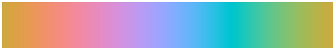
Here’s an Oklab color gradient with varying hue and constant lightness and chroma.
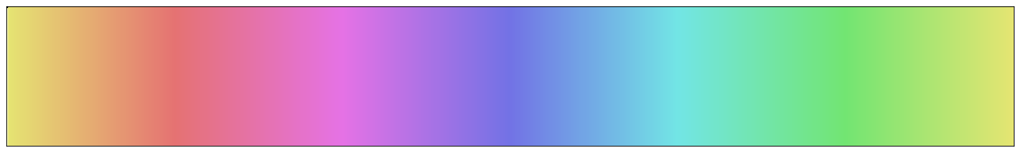
Compare this to a similar plot of a HSV color gradient with varying hue and constant value and saturation (HSV using the sRGB color space).
The gradient is quite uneven and there are clear differences in lightness for different hues. Yellow, magenta and cyan appear much lighter than red and blue.
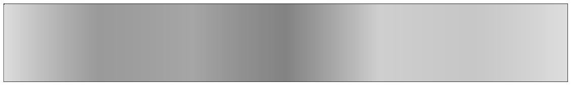
Here is lightness of the HSV plot, as predicted by Oklab:
Implementation
Converting from XYZ to Oklab
Given a color in coordinates, with a D65 whitepoint and white as Y=1, Oklab coordinates can be computed like this:
First the coordinates are converted to an approximate cone responses:
A non-linearity is applied:
Finally, this is transformed into the -coordinates:
with the following values for and :
The inverse operation, going from Oklab to XYZ is done with the following steps:
Table of example XYZ and Oklab pairs
Provided to test Oklab implementations. Computed by transforming the XYZ coordinates to Oklab and rounding to three decimals.
X Y Z L a b 0.950 1.000 1.089 1.000 0.000 0.000 1.000 0.000 0.000 0.450 1.236 -0.019 0.000 1.000 0.000 0.922 -0.671 0.263 0.000 0.000 1.000 0.153 -1.415 -0.449
Converting from linear sRGB to Oklab
Since this will be a common use case, here is the code to convert linear sRGB values to Oklab and back. To compute linear sRGB values, see my previous post.
The code is in C++, but without any fancy features so should be easy to translate. The code is available in public domain, feel free to use it any way you please. It is also available under an MIT licensee if you for some reason can’t or don’t want to use public domain software. The license text is available here
struct Lab {float L; float a; float b;};
struct RGB {float r; float g; float b;};

Lab linear_srgb_to_oklab(RGB c)
{
    float l = 0.4122214708f * c.r + 0.5363325363f * c.g + 0.0514459929f * c.b;
	float m = 0.2119034982f * c.r + 0.6806995451f * c.g + 0.1073969566f * c.b;
	float s = 0.0883024619f * c.r + 0.2817188376f * c.g + 0.6299787005f * c.b;

    float l_ = cbrtf(l);
    float m_ = cbrtf(m);
    float s_ = cbrtf(s);

    return {
        0.2104542553f*l_ + 0.7936177850f*m_ - 0.0040720468f*s_,
        1.9779984951f*l_ - 2.4285922050f*m_ + 0.4505937099f*s_,
        0.0259040371f*l_ + 0.7827717662f*m_ - 0.8086757660f*s_,
    };
}

RGB oklab_to_linear_srgb(Lab c)
{
    float l_ = c.L + 0.3963377774f * c.a + 0.2158037573f * c.b;
    float m_ = c.L - 0.1055613458f * c.a - 0.0638541728f * c.b;
    float s_ = c.L - 0.0894841775f * c.a - 1.2914855480f * c.b;

    float l = l_*l_*l_;
    float m = m_*m_*m_;
    float s = s_*s_*s_;

    return {
		+4.0767416621f * l - 3.3077115913f * m + 0.2309699292f * s,
		-1.2684380046f * l + 2.6097574011f * m - 0.3413193965f * s,
		-0.0041960863f * l - 0.7034186147f * m + 1.7076147010f * s,
    };
}
The matrices were updated 2021-01-25. The new matrices have been derived using a higher precision sRGB matrix and with exactly matching D65 values. The old matrices are available here for reference. The values only differ after the first three decimals.
Depending on use case you might want to use the sRGB matrices your application uses directly instead of the ones provided here.
This is everything you need to use the Oklab color space! If you need a simple perceptual color space, try it out.
The rest of the post will go into why a new color space was needed, how it has been constructed and how it compares with existing color spaces.
Motivation and derivation of Oklab
What properties does a perceptual color space need to satisfy to be useful for image processing? The answer to this is always going to be a bit subjective, but based on my experience, these are a good set of requirements:
- Should be an opponent color space, similar to for example CIELAB.
- Should predict lightness, chroma and hue well. , and should be perceived as orthogonal, so one can be altered without affecting the other two. This is useful for things like turning an image black and white and increasing colorfulness without introducing hue shifts etc.
- Blending two colors should result in even transitions. The transition colors should appear to be in between the blended colors (e.g. passing through a warmer color than either original color is not good).
- Should assume a D65 whitepoint. This is what common color spaces like sRGB, rec2020 and Display P3 uses.
- Should behave well numerically. The model should be easy to compute, numerically stable and differentiable.
- Should assume normal well lit viewing conditions. The complexity of supporting different viewing conditions is not practical in most applications. Information about absolute luminance and background luminance adaptation does not normally exist and the viewing conditions can vary.
- If the scale/exposure of colors are changed, the perceptual coordinates should just be scaled by a factor. To handle a large dynamic range without requiring knowledge of viewing conditions all colors should be modelled as if viewed under normal viewing conditions and as if the eye is adapted to roughly the luminance of the color. This avoids a dependence on scaling.
What about existing models?
Let’s look at existing models and how they stack up against these requirements. Further down there are graphs that illustrate some of these issues.
- CIELAB and CIELUV – Largest issue is their inability to predict hue. In particular blue hues are predicted badly. Other smaller issues exist as well
- CIECAM02-UCS and the newer CAM16-UCS – Does a good job at being perceptually uniform overall, but doesn’t meet other requirements: Bad numerical behavior, it is not scale invariant and blending does not behave well because of its compression of chroma. Hue uniformity is decent, but other models predict it more accurately.
- OSA-UCS – Overall does a good job. The transformation to OSA-UCS lacks an analytical inverse unfortunately which makes it impractical.
- IPT – Does a great job modelling hue uniformity. Doesn’t predict lightness and chroma well unfortunately, but meets all other requirements. Is simple computationally and does not depend on the scale/exposure.
- JzAzBz – Overall does a fairly good job. Designed to have uniform scaling of lightness for HDR data. While useful in some cases this introduces a dependence on the scale/exposure that makes it hard to use in general cases.
- HSV representation of sRGB – Only on this list because it is widely used. Does not meet any of the requirements except having a D65 whitepoint.
So, all in all, all these existing models have drawbacks.
Out of all of these, two models stand out: CAM16-UCS, for being the model with best properties of perceptual uniformity overall, and IPT for having a simple computational structure that meets all the requirements besides predicting lightness and chroma well.
For this reason it is reasonable to try to make a new color space, with the same computational structure as IPT, but that performs closer to CAM16-UCS in terms of predicting lightness and chroma. This exploration resulted in Oklab.
How Oklab was derived
To derive Oklab, three datasets were used:
- A generated data set of pairs of colors with the same lightness but random hue and chroma, generated using CAM16 and normal viewing conditions. Colors were limited to be within Pointer’s Gamut – the set of possible surface colors.
- A generated data set of pairs of colors with the same chroma but random hue and lightness, generated using CAM16 and normal viewing conditions. Colors were limited to be within Pointer’s Gamut
- The uniform perceived hue data used to derive IPT. From this data, colors were combined into pairs of colors with equal perceived hue.
These datasets can be used to test prediction of lightness, chroma and hue respectively. If a color space accurately models , and , then all pairs in lightness dataset should have the same value for , all pairs in the chroma dataset the same value for and all pairs in the hue dataset the same values for .
To test a color space it is not possible to simply check the distance in predictions in the tested color space however, since that will depend on the scaling of the color space. It is also not desirable to exactly predict ground truth values for , and , since it is more important that our model has perceptually orthogonal coordinates, than that the model has the same spacing within each coordinate.
Instead the following approach was used to create an error metric independent of the color space:
- For each dataset all the pairs are converted to the tested color space.
- Coordinates that are supposed to be the same within a pair are swapped to generate a new set of altered pairs:
- For the lightness dataset, the L coordinates are swapped between the pairs, and so on.
- These altered pair would be equal to the original pair if the model predicts the datasets perfectly.
- The perceived distance between the original colors and the altered colors are are computed using CIEDE2000.
- The error for each pair is given as the minimum of the two color differences.
- The error for the entire dataset is the root mean squared error of the color differences.
Oklab was derived by optimizing the parameters of a color space with the same structure as IPT, to get a low error on all the datasets. For completeness, here is the structure of the color space – the parameters to optimize are the 3x3 matrices and and the positive number .
A couple of extra constraints were also added, since this error doesn’t alone determine the scale and orientation of the color model.
- Positive b is oriented to the same yellow color as CAM16
- D65 (normalized with ) should transform to and
- The and plane is scaled so that around 50% gray the ratio of color differences along the lightness axis and the and plane is the same as the ratio for color differences predicted by CIEDE2000.
Using these constraints a fairly good model was found, but based on the results two more changes was made. The value ended up very close to 1/3, 0.323, and when looking at the sRGB gamut, the blue colors folded in on themselves slightly, resulting in a non-convex sRGB gamut. By forcing the value of to 1/3 and adding a constraint the blue colors to not fold inwards, the final Oklab model was derived. The error was not noticeably affected by these restrictions.
Comparison with other color spaces
Here are the errors for the three different datasets across color spaces, given both as root mean square error and as the 95th percentile. The best performing result is highlighted in bold in each row (ignoring CAM16 since it is the origin of the test data). Since the lightness and chroma data was generated using CAM16 rather than being data from experiments, this data can’t be used to say which model best matches human perception. What can be said is that Oklab does a good job at predicting hue and its predictions for chroma and lightness are close to those of CAM16-UCS.
| Oklab | CIELAB | CIELUV | OSA-UCS | IPT | JzAzBz | HSV | CAM16-UCS | |
|---|---|---|---|---|---|---|---|---|
| L RMS | 0.20 | 1.70 | 1.72 | 2.05 | 4.92 | 2.38 | 11.59 | 0.00 |
| C RMS | 0.81 | 1.84 | 2.32 | 1.28 | 2.18 | 1.79 | 3.38 | 0.00 |
| H RMS | 0.49 | 0.69 | 0.68 | 0.49 | 0.48 | 0.43 | 1.10 | 0.59 |
| L 95 | 0.44 | 3.16 | 3.23 | 4.04 | 9.89 | 4.55 | 23.17 | 0.00 |
| C 95 | 1.78 | 3.96 | 5.03 | 2.73 | 4.64 | 3.77 | 7.51 | 0.00 |
| H 95 | 1.06 | 1.56 | 1.51 | 1.08 | 1.02 | 0.92 | 2.42 | 1.31 |
To be able to include HSV in these comparisons, a Lab-like color space has been defined based on it, by interpreting HSV as a cylindrical color space and converting to a regular grid.
JzAzBz has been used with white scaled so that Y=100. This matches the graphs in the original paper, but it is unclear if this is how it is intended to be used. (See this colorio Github issue for a discussion of the topic)
Munsell data
Here is Munsell color chart data (with V=5) plotted in the various color spaces. If a color space has a chroma prediction that matches that of the Munsell data, the rings formed by the data should appear as perfect circles. The quality of this data is a bit hard to assess, since it isn’t directly using experimental data, it is a color chart created from experimental data back in the 1940s.
Oklab and CAM16-UCS seem to predict the Munsell data well, while other spaces squash the circles in the dataset in various ways, which would indicate that Oklab does a better job than most of the color spaces of predicting chroma.
Oklab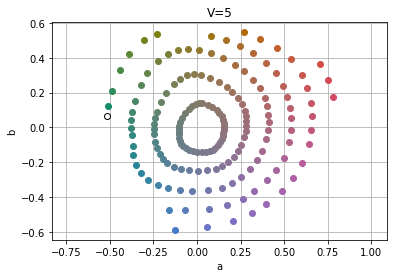
CIELAB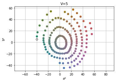
CIELUV
OSA-UCS
IPT
JzAzBz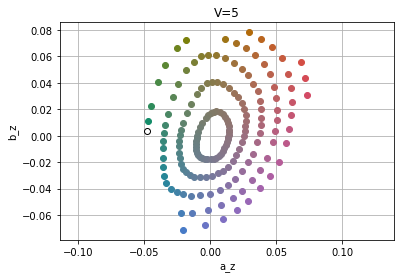
HSV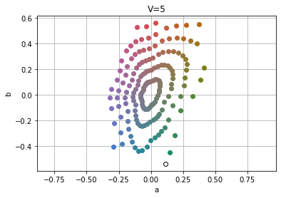
CAM16-UCS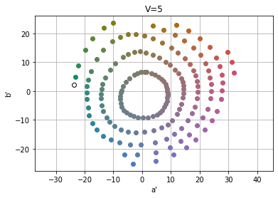
Luo-Rigg dataset and full gamut
These plots show three things, ellipses, scaled based on perception of color differences from the Luo-Rigg dataset, the shape of the full visible gamut (the black line corresponds to pure single wavelength lights) and a slice of the sRGB gamut.
A few interesting observations are:
- The shape of the full gamut is quite odd in CIELAB and OSA-UCS, which likely means that their predictions are quite bad for highly saturated colors
- Except for CAM16-UCS the ellipses are stretched out as chroma increases. CAM16 explicitly compresses chroma to better match experimental data, which makes this data look good, but makes color blending worse
Oklab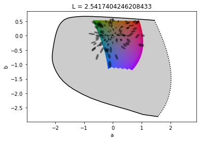
CIELAB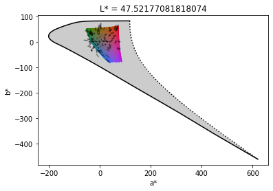
CIELUV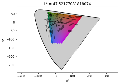
OSA-UCS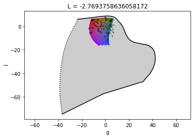
IPT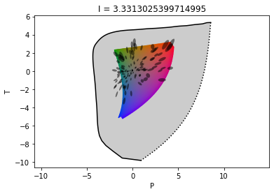
JzAzBz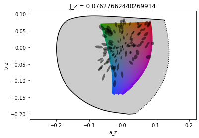
HSV
Data missing. Plot broken since HSV does not handle colors outside sRGB gamut
CAM16-UCS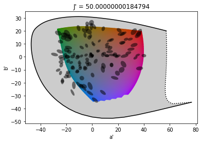
Blending colors
Here are plots of white blended with a blue color, using the various color spaces tested. The blue color has been picked since it is the hue with the most variation between spaces. CIELAB, CIELUV and HSV all show hue shifts towards purple. CAM16 has a different issue, with the color becoming desaturated quickly, resulting in a transition that doesn’t look as even as some of the other ones.
Oklab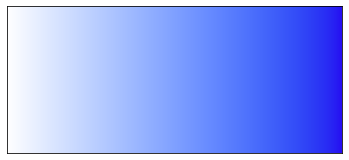
CIELAB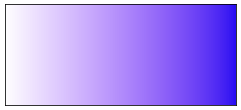
CIELUV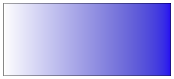
OSA-UCS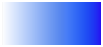
IPT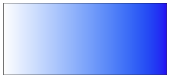
JzAzBz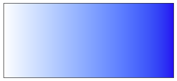
HSV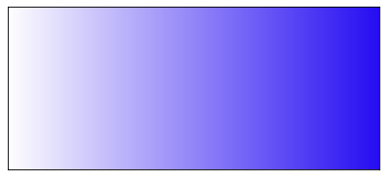
CAM16-UCS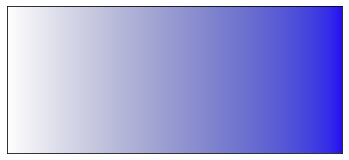
Conclusion
This post has introduced the Oklab color space, a perceptual color space for image processing. Oklab is able to predict perceived lightness, chroma and hue well, while being simple and well-behaved numerically and easy to adopt.
In future posts I want to look into using Oklab to build a better perceptual color picker and more.
Oklab and the images in this post have been made using python, jupyter, numpy, scipy matplotlib, colorio and colour.
If you liked this article, it would be great if you considered sharing it:
For discussions and feedback, ping me on Twitter.
Published