sRGB gamut clipping
When doing image processing, rendering or converting between RGB color spaces, it is easy to end up with RGB values outside of the 0.0 to 1.0 range (or 0 to 255 for 8-bit colors). This normally means that it isn’t possible to encode the color and it needs to be adjusted somehow before being displayed or encoded (scRGB is an example of an exception, and has a different range). The range of supported colors in a color spaces is referred to as a its gamut.
Many of the colors outside the gamut are still valid colors, they just can’t be encoded in the given color space. The colors that can’t be encoded can be categorized as follows (for RGB color spaces without imaginary primaries):
- One or more RGB values are larger than one, but none are negative
These colors are too bright for the color space, but could be encoded at a lower luminance. - One or more negative values
These color are more colorful than the color space is able to encode. Some of these can be real colors, but they can also be colors more colorful than physically possible. This is a consequence of linear encoding of colors, which is able to encode colors that can’t exist in real life.
The simplest technique for dealing with colors outside the valid range is to simply clamp , and individually. The simplicity of this makes the technique widespread, but unfortunately it has significant drawbacks and can lead to unpleasant color distortions.
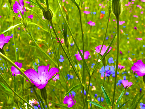
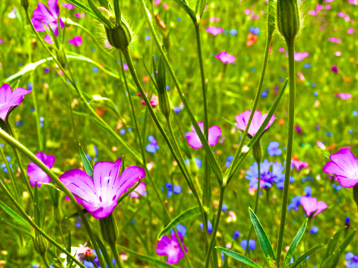
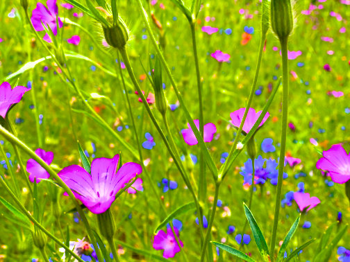
Here is an example of taking a photo and increasing its exposure and colorfulness significantly, with results displayed as sRGB. Colorfulness has been increased by scaling Oklab chroma. RGB values here are simply clamped to the 0.0 to 1.0 range.
 Unprocessed
 Processed with out of range values clamped
This is of course problematic. Hues are heavily distorted and all the details in the flowers are gone. Better methods are needed. Thankfully, this problem isn’t new and has been researched a lot over the years.
Two main research topics exist:
Tone mapping, which is concerned with mapping high dynamic range images to a lower dynamic range. This typically involves altering both colors inside and outside the gamut and sometimes involves different kinds of spatial filtering to keep details while reducing overall dynamic range.
Gamut mapping, which is concerned with mapping colors from one color space to another and dealing with the mismatch in what colors can be encoded. This can either be done using gamut compression or gamut expansion, which adjusts all colors of an image, or using gamut clipping, which leaves colors that exist in both color spaces intact, while mapping colors outside the gamut back in range. For an overview see the paper “The Fundamentals of Gamut Mapping: A Survey”.
Tone mapping, gamut expansion and gamut compression are all useful techniques, but will not be the focus of this article. Instead we will limit the scope to creating a practical alternative to clipping sRGB values, by looking at gamut clipping in the sRGB color space and on relatively simple, robust and portable algorithms. The source code for the operations shown is also available, at the end of the article.
The techniques investigated are also, with some additional work, applicable to other color spaces, and some of the building blocks can be for other things, such as gamut compression. Combining gamut clipping with tone mapping can also be useful since some tone mapping techniques may still produce colors outside the target gamut.
Gamut Clipping
The goal of gamut clipping is to take colors that are outside the target gamut, and map them back to valid colors in a way that avoids perceived distortion and artifacts. In this article we also want to do this in a way that is reasonably efficient and simple to implement. Many techniques require complex iterative algorithms per pixel (or storing the results in 3D lookup tables) – those will not be considered here, but can be useful for many applications.
Instead we will take this commonly used approach:
- Work in a perceptual color space.
- Keep hue constant, only change lightness and chroma.
- Only project color along straight lines in the perceptual color space.
For an overview of different approaches, see the paper The Fundamentals of Gamut Mapping: A Survey.
As a color space, we will use the Oklab perceptual color space, since it models hue, chroma and lightness well while being easy to work with mathematically. In particular, with Oklab, the shape of the gamut of an RGB color space is described by cubic polynomials, which are quite practical to work with compared to the equations you get with other spaces.
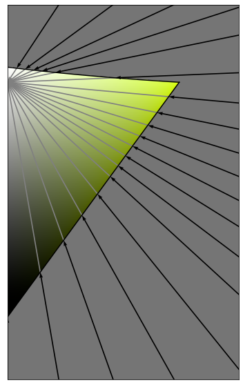
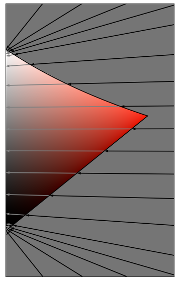
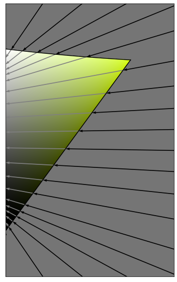
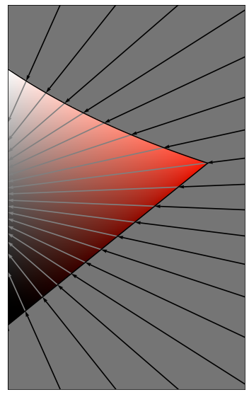
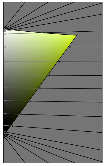
Since we have decided to keep hue constant, it is now possible to plot the problem in two dimensions, using lightness, , and chroma, . To better understand the shape of the sRGB gamut, let’s look at of slices of constant hue. These are sampled every 30 degrees:
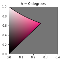
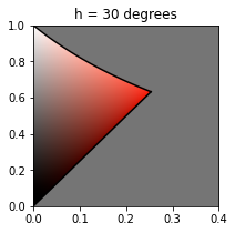
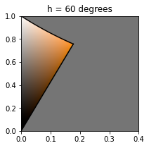
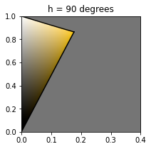
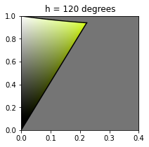
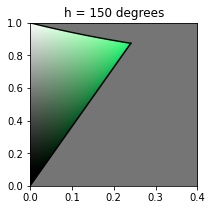
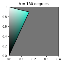
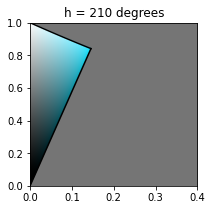
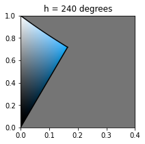
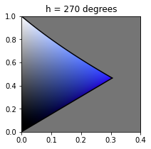
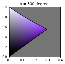
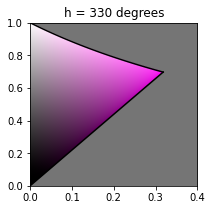
Our goal is to find a way to map colors outside the gamut, shown in grey in the graphs, back into the gamut using straight lines. This problem can be split into two parts:
- Deciding along which line to project the color onto the gamut
- Finding the intersection between the line and the gamut
Lets start by tackling part 2.
Intersecting lines with the gamut
The math here is quite involved, so this sections just contains an overview of the approach. If that is still too much math, skip to the next section. For more details, see the source code.
Expressed mathematically, the problem we want to solve is: Given a color expressed as and , and a point that is known to be inside the gamut, we want to find a value so that is a point on the gamut surface. We will also set since the projections we want to make later always pass through the axis.
Using the definition of Oklab here, we get this conversion from to linear :
The gamut is then defined by the following inequalities:
This is enough information to solve the problem numerically, but involves solving six cubic polynomials. We are after a faster solution that uses more knowledge about the problem.
By studying the gamut graphs and the equations, we can draw a few conclusions:
- For a given hue, the lower limit is always a straight line passing through
- The gamut shape is always close to a triangle, with two of its corners in and
- If we can find the third point, we know exactly the lower limit and we have good first approximation of the upper limit
The location of the third point, , , only depends on . To find it we use a fitted numerical approximation followed by a single step of Halley’s method, this gives an error less than (except for one point where the derivative is close to infinite). Since this only depends on it is also possible to use a 1D lookup table for it.
With the location for the cusp, it is now possible to find the intersection with the triangle. If the intersection is with the lower edge, this is everything we need to do. If the intersection is with the upper half, the triangle is only an approximation and we need to refine the solution. Again, one step of Halley’s method is enough to do this with high accuracy.
Altogether, this is everything needed to find the intersection between a line and the sRGB gamut. To derive the numerical approximation of the location of the cusp, this Google Colab Notebook was used. With same method is should be possible derive approximations for other RGB color spaces. The complete source code is available at the end of this article.
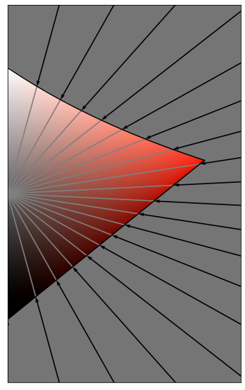
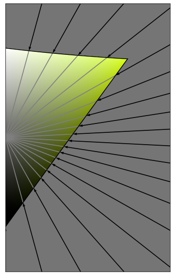
Choosing which line to project along
Starting with a point , we want to decide a point within the gamut to project towards. The choice is a matter of preference and can depend on context.
Let’s start by testing a few simple existing methods and see what the projections look like for different hue slices and when applied the test image from the beginning.
Keep lightness constant, only compress chroma
Lightness is kept constant if it is between zero and one, otherwise it is clamped. This is done by projecting towards


 Gamut clipping test
Projection towards a single point, hue independent
Colors are projected towards the middle of the valid greyscale colors:
 Gamut clipping test
Projection towards a single point, hue dependent
Colors are projected towards the lightness of the cusp of the gamut for the current hue:

 Gamut clipping test
Can we do better?
The choice of projection will always be a matter of preference. Overall I think preserving lightness does the best overall of the above methods (and others agree, it is a commonly used technique). One challenge with preserving lightness though is that all colors with or get projected to a single point, and that highly saturated colors can become almost completely desaturated if light or dark enough, even though sacrificing just a small amount of lightness would have resulted in a much closer match.
For this reason I’ve looked into creating new methods that mostly preserve lightness, but behaves closer to the single point projection methods for high and low lightness colors. The result is two new methods. They are novel as far as I am aware, but there are a lot of gamut mapping papers I haven’t read.
The first method is based on projection towards and the second based on . Both have a parameter to control to what extent lightness is preserved. is a real number larger than 0, where values close to zero will behave as pure chroma compression, and larger values will behave closer to the single point projection methods. Here is an overview of the two methods:
Adaptive , hue independent
This method blends between pure chroma compression and projection towards a single point, .
is computed with the following equations:
Here are some results with different values for :

 Gamut clipping test

 Gamut clipping test

 Gamut clipping test
Adaptive , hue dependent
This method blends between pure chroma compression and projection towards a single point,
is computed with the following equations:
Here are some results with different values for :

 Gamut clipping test

 Gamut clipping test


 Gamut clipping test
Results
The following images compare RGB clipping with the five different gamut clipping methods above and a few choices of , across different images. All images have had their colorfulness increased by scaling Oklab chroma and their exposure increased slightly.
The processing done here is for testing purposes only. I would not recommend doing image processing that creates this many invalid colors and solving it by gamut clipping. For example, in cases like this, some kind of gamut compressions would probably be a better choice.
All the original photos are by me and both original images and the results are licensed under CC BY-SA.
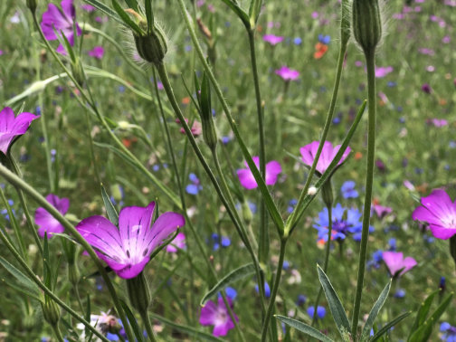
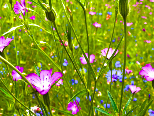
Flowers
Unprocessed
 Colors in gamut
RGB clipped
Chroma clipped
projection
projection
Adaptive ,
Adaptive ,
Adaptive ,
Adaptive ,
Adaptive ,
Adaptive ,
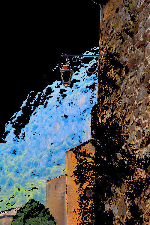
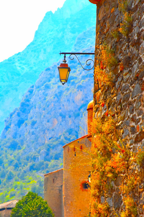
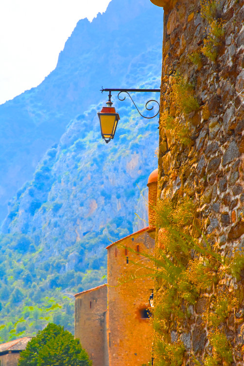
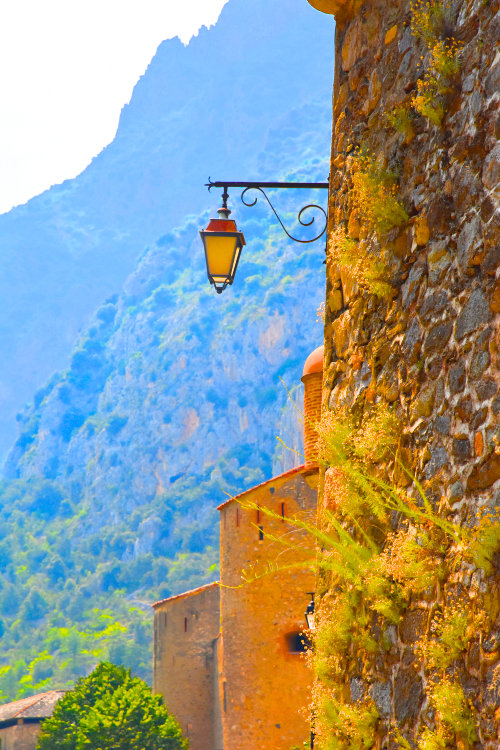
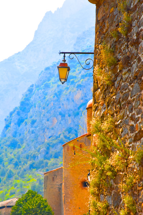
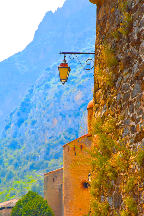
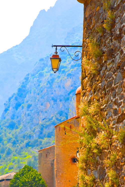
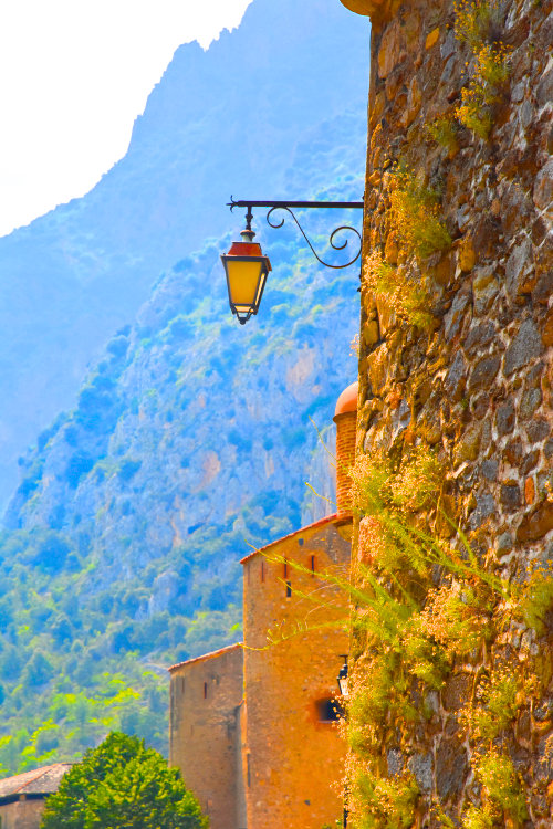
Lamp
 Unprocessed
 Colors in gamut
 RGB clipped
 Chroma clipped
 projection
 projection
 Adaptive ,
 Adaptive ,
 Adaptive ,
 Adaptive ,
 Adaptive ,
 Adaptive ,
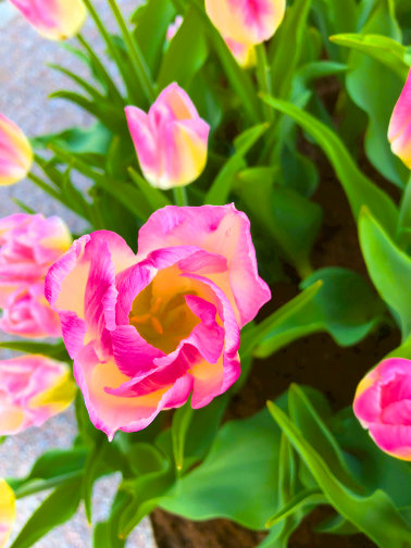
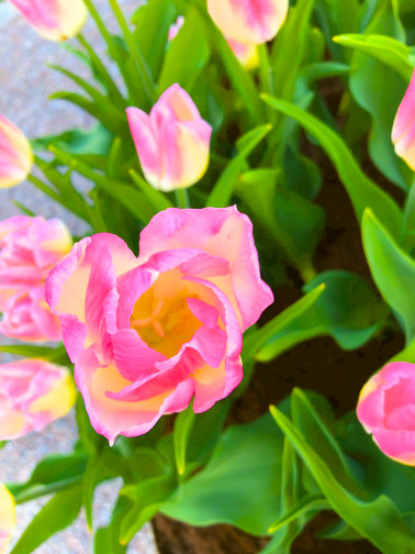
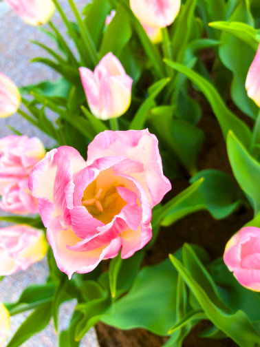
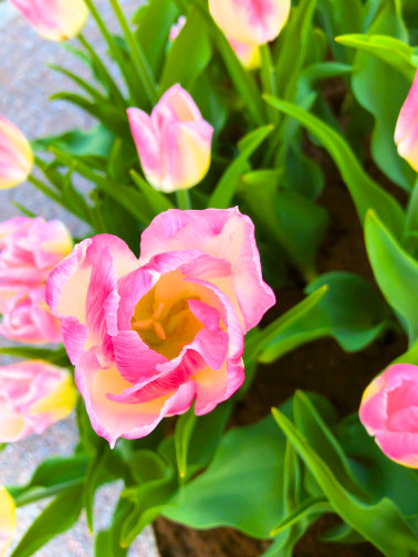
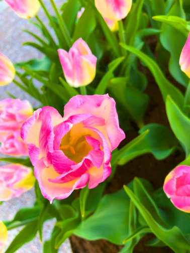
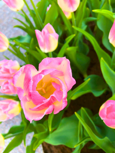
Tulip
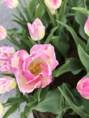 Unprocessed
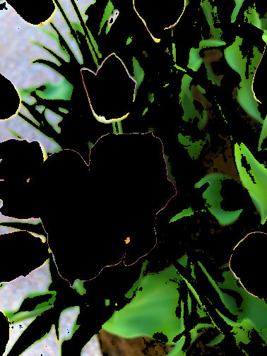 Colors in gamut
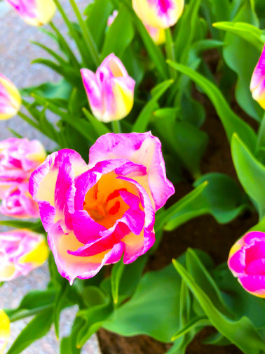 RGB clipped
 Chroma clipped
 projection
 projection
 Adaptive ,
 Adaptive ,
 Adaptive ,
 Adaptive ,
 Adaptive ,
 Adaptive ,
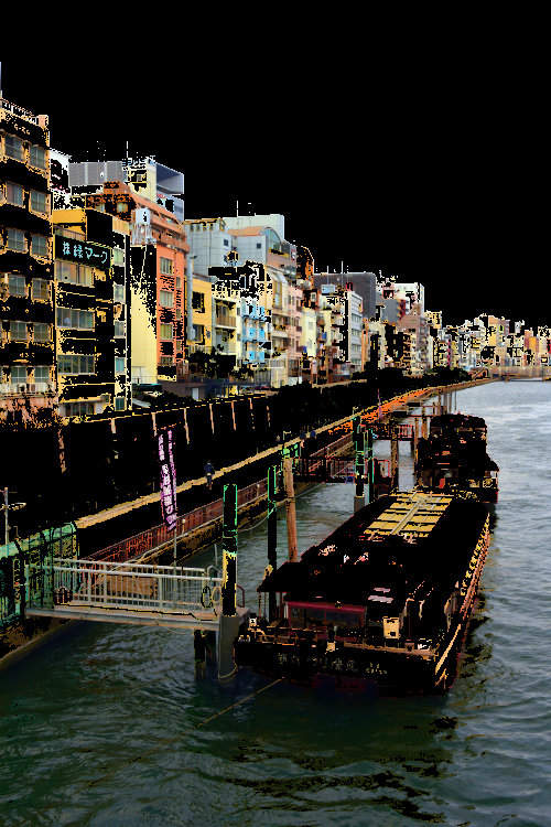
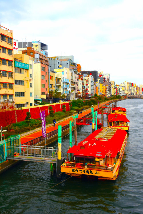
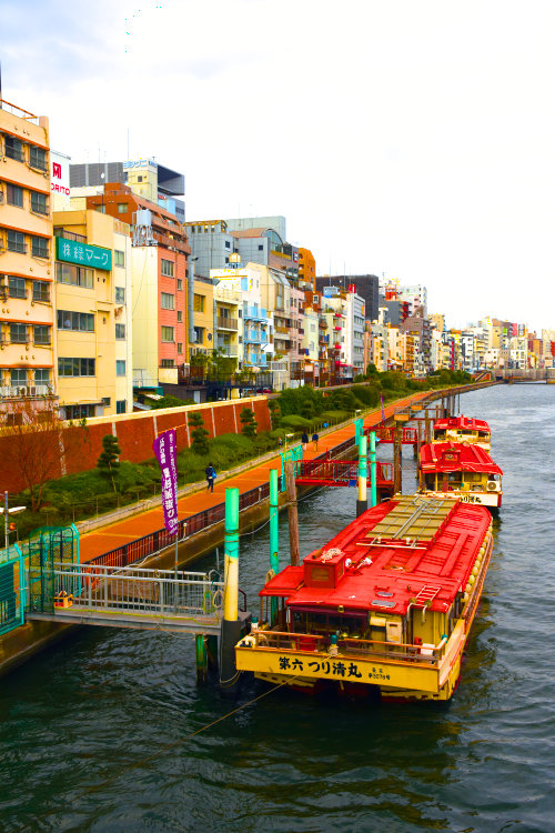
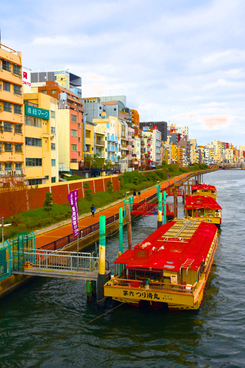
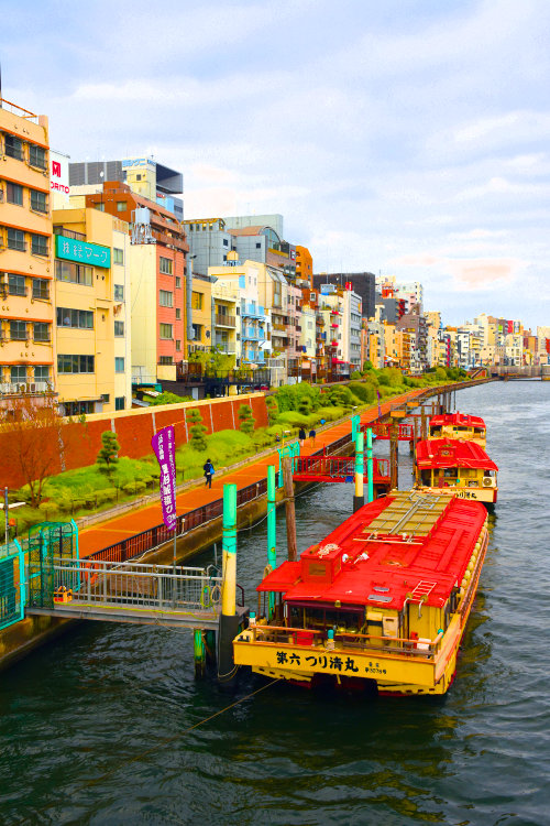
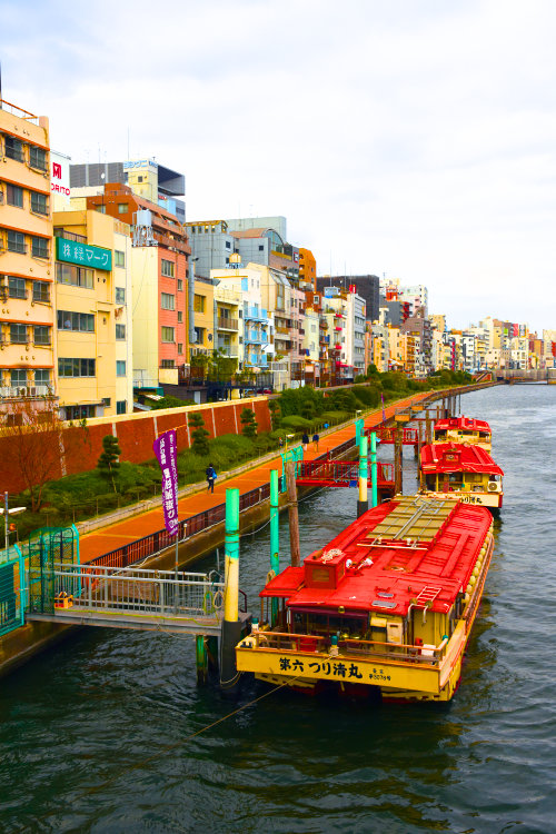
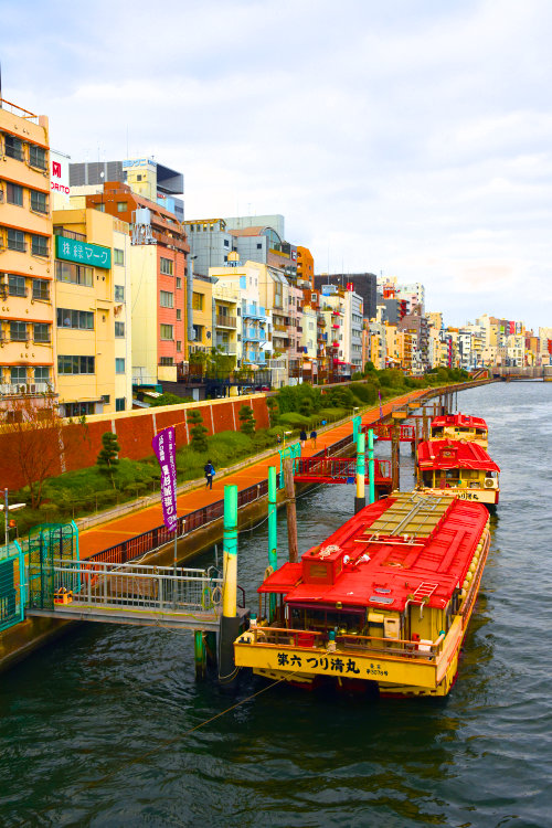
Boat
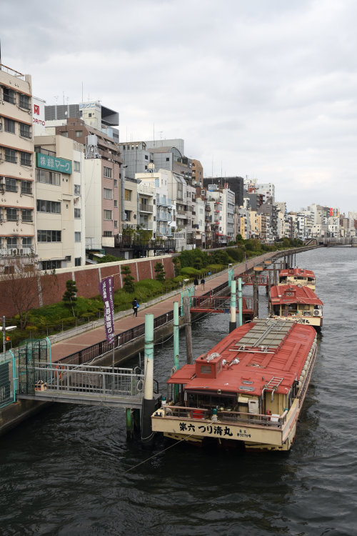 Unprocessed
 Colors in gamut
 RGB clipped
 Chroma clipped
 projection
 projection
 Adaptive ,
 Adaptive ,
 Adaptive ,
 Adaptive ,
 Adaptive ,
 Adaptive ,
Conclusions and future work
Overall, doing gamut clipping using Oklab seems like a useful tool, and is fairly easy to implement. The results here though are not enough to determine how it compares with other algorithm or how results are perceived if comparing wide gamut images with clipped versions. Doing more studies and comparisons would be interesting. In particular, should compare the results against methods more complex methods that minimize color distances, such as the ones evaluated in the paper: “Gamut Mapping for Digital Cinema”
Personally, of the methods evaluated here, I think a good default choice would be adaptive with , but in specific cases other methods and values can definitely perform better. At the choice between and seems to matter very little visually. is then preferable, since it is cheaper to compute, and can be implemented with a single 2D lookup table if desired (From hue and to and ).
There is also a lot of potential future work:
- Would be nice with a solution that could work directly with RGB matrices, instead of optimizing some constants separately. This way a solutions could be created quickly for any RGB color space.
- One issue, that is related to the sRGB gamut rather than the clipping algorithm, is the sharp ridges of high chroma that sometimes get created. A smoothed version of the sRGB gamut could be interesting to clip to instead, producing a more even blend at the expense of some of the highly saturated colors.
- There are also a lot of other applications for intersecting lines with the gamut to explore.
My next post will be about creating HSV and HSL like color pickers with improved uniformity, utilizing the gamut intersection algorithm described here.
Source code
All the source code on this page is provided under the MIT license:
Copyright (c) 2021 Björn Ottosson

Permission is hereby granted, free of charge, to any person obtaining a copy of
this software and associated documentation files (the "Software"), to deal in
the Software without restriction, including without limitation the rights to
use, copy, modify, merge, publish, distribute, sublicense, and/or sell copies
of the Software, and to permit persons to whom the Software is furnished to do
so, subject to the following conditions:

The above copyright notice and this permission notice shall be included in all
copies or substantial portions of the Software.

THE SOFTWARE IS PROVIDED "AS IS", WITHOUT WARRANTY OF ANY KIND, EXPRESS OR
IMPLIED, INCLUDING BUT NOT LIMITED TO THE WARRANTIES OF MERCHANTABILITY,
FITNESS FOR A PARTICULAR PURPOSE AND NONINFRINGEMENT. IN NO EVENT SHALL THE
AUTHORS OR COPYRIGHT HOLDERS BE LIABLE FOR ANY CLAIM, DAMAGES OR OTHER
LIABILITY, WHETHER IN AN ACTION OF CONTRACT, TORT OR OTHERWISE, ARISING FROM,
OUT OF OR IN CONNECTION WITH THE SOFTWARE OR THE USE OR OTHER DEALINGS IN THE
SOFTWARE.
Oklab to linear sRGB conversion
Linear sRGB to Oklab conversion, identical to the the Oklab blog post.
This is using linear sRGB values in the range 0.0 to 1.0. To compute linear sRGB values, see my previous post.
struct Lab {float L; float a; float b;};
struct RGB {float r; float g; float b;};

Lab linear_srgb_to_oklab(RGB c)
{
	float l = 0.4122214708f * c.r + 0.5363325363f * c.g + 0.0514459929f * c.b;
	float m = 0.2119034982f * c.r + 0.6806995451f * c.g + 0.1073969566f * c.b;
	float s = 0.0883024619f * c.r + 0.2817188376f * c.g + 0.6299787005f * c.b;

	float l_ = cbrtf(l);
	float m_ = cbrtf(m);
	float s_ = cbrtf(s);

	return {
		0.2104542553f * l_ + 0.7936177850f * m_ - 0.0040720468f * s_,
		1.9779984951f * l_ - 2.4285922050f * m_ + 0.4505937099f * s_,
		0.0259040371f * l_ + 0.7827717662f * m_ - 0.8086757660f * s_,
	};
}

RGB oklab_to_linear_srgb(Lab c)
{
    float l_ = c.L + 0.3963377774f * c.a + 0.2158037573f * c.b;
    float m_ = c.L - 0.1055613458f * c.a - 0.0638541728f * c.b;
    float s_ = c.L - 0.0894841775f * c.a - 1.2914855480f * c.b;

    float l = l_ * l_ * l_;
    float m = m_ * m_ * m_;
    float s = s_ * s_ * s_;

    return {
        +4.0767416621f * l - 3.3077115913f * m + 0.2309699292f * s,
        -1.2684380046f * l + 2.6097574011f * m - 0.3413193965f * s,
        -0.0041960863f * l - 0.7034186147f * m + 1.7076147010f * s,
    };
}
Intersection with sRGB gamut
Implementations of the sRGB gamut intersection algorithm. The code has been written to be easy to follow. Consider optimizing for your use case.
// Finds the maximum saturation possible for a given hue that fits in sRGB
// Saturation here is defined as S = C/L
// a and b must be normalized so a^2 + b^2 == 1
float compute_max_saturation(float a, float b)
{
    // Max saturation will be when one of r, g or b goes below zero.

    // Select different coefficients depending on which component goes below zero first
    float k0, k1, k2, k3, k4, wl, wm, ws;

    if (-1.88170328f * a - 0.80936493f * b > 1)
    {
        // Red component
        k0 = +1.19086277f; k1 = +1.76576728f; k2 = +0.59662641f; k3 = +0.75515197f; k4 = +0.56771245f;
        wl = +4.0767416621f; wm = -3.3077115913f; ws = +0.2309699292f;
    }
    else if (1.81444104f * a - 1.19445276f * b > 1)
    {
        // Green component
        k0 = +0.73956515f; k1 = -0.45954404f; k2 = +0.08285427f; k3 = +0.12541070f; k4 = +0.14503204f;
        wl = -1.2684380046f; wm = +2.6097574011f; ws = -0.3413193965f;
    }
    else
    {
        // Blue component
        k0 = +1.35733652f; k1 = -0.00915799f; k2 = -1.15130210f; k3 = -0.50559606f; k4 = +0.00692167f;
        wl = -0.0041960863f; wm = -0.7034186147f; ws = +1.7076147010f;
    }

    // Approximate max saturation using a polynomial:
    float S = k0 + k1 * a + k2 * b + k3 * a * a + k4 * a * b;

    // Do one step Halley's method to get closer
    // this gives an error less than 10e6, except for some blue hues where the dS/dh is close to infinite
    // this should be sufficient for most applications, otherwise do two/three steps

    float k_l = +0.3963377774f * a + 0.2158037573f * b;
    float k_m = -0.1055613458f * a - 0.0638541728f * b;
    float k_s = -0.0894841775f * a - 1.2914855480f * b;

    {
        float l_ = 1.f + S * k_l;
        float m_ = 1.f + S * k_m;
        float s_ = 1.f + S * k_s;

        float l = l_ * l_ * l_;
        float m = m_ * m_ * m_;
        float s = s_ * s_ * s_;

        float l_dS = 3.f * k_l * l_ * l_;
        float m_dS = 3.f * k_m * m_ * m_;
        float s_dS = 3.f * k_s * s_ * s_;

        float l_dS2 = 6.f * k_l * k_l * l_;
        float m_dS2 = 6.f * k_m * k_m * m_;
        float s_dS2 = 6.f * k_s * k_s * s_;

        float f  = wl * l     + wm * m     + ws * s;
        float f1 = wl * l_dS  + wm * m_dS  + ws * s_dS;
        float f2 = wl * l_dS2 + wm * m_dS2 + ws * s_dS2;

        S = S - f * f1 / (f1*f1 - 0.5f * f * f2);
    }

    return S;
}

// finds L_cusp and C_cusp for a given hue
// a and b must be normalized so a^2 + b^2 == 1
struct LC { float L; float C; };
LC find_cusp(float a, float b)
{
	// First, find the maximum saturation (saturation S = C/L)
	float S_cusp = compute_max_saturation(a, b);

	// Convert to linear sRGB to find the first point where at least one of r,g or b >= 1:
	RGB rgb_at_max = oklab_to_linear_srgb({ 1, S_cusp * a, S_cusp * b });
	float L_cusp = cbrtf(1.f / max(max(rgb_at_max.r, rgb_at_max.g), rgb_at_max.b));
	float C_cusp = L_cusp * S_cusp;

	return { L_cusp , C_cusp };
}

// Finds intersection of the line defined by
// L = L0 * (1 - t) + t * L1;
// C = t * C1;
// a and b must be normalized so a^2 + b^2 == 1
float find_gamut_intersection(float a, float b, float L1, float C1, float L0)
{
	// Find the cusp of the gamut triangle
	LC cusp = find_cusp(a, b);

	// Find the intersection for upper and lower half seprately
	float t;
	if (((L1 - L0) * cusp.C - (cusp.L - L0) * C1) <= 0.f)
	{
		// Lower half

		t = cusp.C * L0 / (C1 * cusp.L + cusp.C * (L0 - L1));
	}
	else
	{
		// Upper half

		// First intersect with triangle
		t = cusp.C * (L0 - 1.f) / (C1 * (cusp.L - 1.f) + cusp.C * (L0 - L1));

		// Then one step Halley's method
		{
			float dL = L1 - L0;
			float dC = C1;

			float k_l = +0.3963377774f * a + 0.2158037573f * b;
			float k_m = -0.1055613458f * a - 0.0638541728f * b;
			float k_s = -0.0894841775f * a - 1.2914855480f * b;

			float l_dt = dL + dC * k_l;
			float m_dt = dL + dC * k_m;
			float s_dt = dL + dC * k_s;


			// If higher accuracy is required, 2 or 3 iterations of the following block can be used:
			{
				float L = L0 * (1.f - t) + t * L1;
				float C = t * C1;

				float l_ = L + C * k_l;
				float m_ = L + C * k_m;
				float s_ = L + C * k_s;

				float l = l_ * l_ * l_;
				float m = m_ * m_ * m_;
				float s = s_ * s_ * s_;

				float ldt = 3 * l_dt * l_ * l_;
				float mdt = 3 * m_dt * m_ * m_;
				float sdt = 3 * s_dt * s_ * s_;

				float ldt2 = 6 * l_dt * l_dt * l_;
				float mdt2 = 6 * m_dt * m_dt * m_;
				float sdt2 = 6 * s_dt * s_dt * s_;

				float r = 4.0767416621f * l - 3.3077115913f * m + 0.2309699292f * s - 1;
				float r1 = 4.0767416621f * ldt - 3.3077115913f * mdt + 0.2309699292f * sdt;
				float r2 = 4.0767416621f * ldt2 - 3.3077115913f * mdt2 + 0.2309699292f * sdt2;

				float u_r = r1 / (r1 * r1 - 0.5f * r * r2);
				float t_r = -r * u_r;

				float g = -1.2684380046f * l + 2.6097574011f * m - 0.3413193965f * s - 1;
				float g1 = -1.2684380046f * ldt + 2.6097574011f * mdt - 0.3413193965f * sdt;
				float g2 = -1.2684380046f * ldt2 + 2.6097574011f * mdt2 - 0.3413193965f * sdt2;

				float u_g = g1 / (g1 * g1 - 0.5f * g * g2);
				float t_g = -g * u_g;

				float b = -0.0041960863f * l - 0.7034186147f * m + 1.7076147010f * s - 1;
				float b1 = -0.0041960863f * ldt - 0.7034186147f * mdt + 1.7076147010f * sdt;
				float b2 = -0.0041960863f * ldt2 - 0.7034186147f * mdt2 + 1.7076147010f * sdt2;

				float u_b = b1 / (b1 * b1 - 0.5f * b * b2);
				float t_b = -b * u_b;

				t_r = u_r >= 0.f ? t_r : FLT_MAX;
				t_g = u_g >= 0.f ? t_g : FLT_MAX;
				t_b = u_b >= 0.f ? t_b : FLT_MAX;

				t += min(t_r, min(t_g, t_b));
			}
		}
	}

	return t;
}
Gamut clipping
Implementations of the gamut clipping methods in this article. The code has been written to be easy to follow. Consider optimizing for your use case.
float clamp(float x, float min, float max)
{
	if (x < min)
		return min;
	if (x > max)
		return max;

	return x;
}

float sgn(float x)
{
	return (float)(0.f < x) - (float)(x < 0.f);
}

RGB gamut_clip_preserve_chroma(RGB rgb)
{
	if (rgb.r < 1 && rgb.g < 1 && rgb.b < 1 && rgb.r > 0 && rgb.g > 0 && rgb.b > 0)
		return rgb;

	Lab lab = linear_srgb_to_oklab(rgb);

	float L = lab.L;
	float eps = 0.00001f;
	float C = max(eps, sqrtf(lab.a * lab.a + lab.b * lab.b));
	float a_ = lab.a / C;
	float b_ = lab.b / C;

	float L0 = clamp(L, 0, 1);

	float t = find_gamut_intersection(a_, b_, L, C, L0);
	float L_clipped = L0 * (1 - t) + t * L;
	float C_clipped = t * C;

	return oklab_to_linear_srgb({ L_clipped, C_clipped * a_, C_clipped * b_ });
}

RGB gamut_clip_project_to_0_5(RGB rgb)
{
	if (rgb.r < 1 && rgb.g < 1 && rgb.b < 1 && rgb.r > 0 && rgb.g > 0 && rgb.b > 0)
		return rgb;

	Lab lab = linear_srgb_to_oklab(rgb);

	float L = lab.L;
	float eps = 0.00001f;
	float C = max(eps, sqrtf(lab.a * lab.a + lab.b * lab.b));
	float a_ = lab.a / C;
	float b_ = lab.b / C;

	float L0 = 0.5;

	float t = find_gamut_intersection(a_, b_, L, C, L0);
	float L_clipped = L0 * (1 - t) + t * L;
	float C_clipped = t * C;

	return oklab_to_linear_srgb({ L_clipped, C_clipped * a_, C_clipped * b_ });
}

RGB gamut_clip_project_to_L_cusp(RGB rgb)
{
	if (rgb.r < 1 && rgb.g < 1 && rgb.b < 1 && rgb.r > 0 && rgb.g > 0 && rgb.b > 0)
		return rgb;

	Lab lab = linear_srgb_to_oklab(rgb);

	float L = lab.L;
	float eps = 0.00001f;
	float C = max(eps, sqrtf(lab.a * lab.a + lab.b * lab.b));
	float a_ = lab.a / C;
	float b_ = lab.b / C;

	// The cusp is computed here and in find_gamut_intersection, an optimized solution would only compute it once.
	LC cusp = find_cusp(a_, b_);

	float L0 = cusp.L;

	float t = find_gamut_intersection(a_, b_, L, C, L0);

	float L_clipped = L0 * (1 - t) + t * L;
	float C_clipped = t * C;

	return oklab_to_linear_srgb({ L_clipped, C_clipped * a_, C_clipped * b_ });
}

RGB gamut_clip_adaptive_L0_0_5(RGB rgb, float alpha = 0.05f)
{
	if (rgb.r < 1 && rgb.g < 1 && rgb.b < 1 && rgb.r > 0 && rgb.g > 0 && rgb.b > 0)
		return rgb;

	Lab lab = linear_srgb_to_oklab(rgb);

	float L = lab.L;
	float eps = 0.00001f;
	float C = max(eps, sqrtf(lab.a * lab.a + lab.b * lab.b));
	float a_ = lab.a / C;
	float b_ = lab.b / C;

	float Ld = L - 0.5f;
	float e1 = 0.5f + fabs(Ld) + alpha * C;
	float L0 = 0.5f*(1.f + sgn(Ld)*(e1 - sqrtf(e1*e1 - 2.f *fabs(Ld))));

	float t = find_gamut_intersection(a_, b_, L, C, L0);
	float L_clipped = L0 * (1.f - t) + t * L;
	float C_clipped = t * C;

	return oklab_to_linear_srgb({ L_clipped, C_clipped * a_, C_clipped * b_ });
}

RGB gamut_clip_adaptive_L0_L_cusp(RGB rgb, float alpha = 0.05f)
{
	if (rgb.r < 1 && rgb.g < 1 && rgb.b < 1 && rgb.r > 0 && rgb.g > 0 && rgb.b > 0)
		return rgb;

	Lab lab = linear_srgb_to_oklab(rgb);

	float L = lab.L;
	float eps = 0.00001f;
	float C = max(eps, sqrtf(lab.a * lab.a + lab.b * lab.b));
	float a_ = lab.a / C;
	float b_ = lab.b / C;

	// The cusp is computed here and in find_gamut_intersection, an optimized solution would only compute it once.
	LC cusp = find_cusp(a_, b_);

	float Ld = L - cusp.L;
	float k = 2.f * (Ld > 0 ? 1.f - cusp.L : cusp.L);

	float e1 = 0.5f*k + fabs(Ld) + alpha * C/k;
	float L0 = cusp.L + 0.5f * (sgn(Ld) * (e1 - sqrtf(e1 * e1 - 2.f * k * fabs(Ld))));

	float t = find_gamut_intersection(a_, b_, L, C, L0);
	float L_clipped = L0 * (1.f - t) + t * L;
	float C_clipped = t * C;

	return oklab_to_linear_srgb({ L_clipped, C_clipped * a_, C_clipped * b_ });
}
If you liked this article, it would be great if you considered sharing it:
For discussions and feedback, ping me on Twitter.
Published